HIGHLIGHTED ARTICLE INVESTIGATION
Penalized Multimarker
vs.
Single-Marker Regression
Methods for Genome-Wide Association Studies of
Quantitative Traits
Hui Yi,*,†Patrick Breheny,‡Netsanet Imam,* Yongmei Liu,§and Ina Hoeschele*,**,1 *Virginia Bioinformatics Institute,†Ph.D. Program in Genetics, Bioinformatics, and Computational Biology, and **Department of Statistics, Virginia Tech University, Blacksburg, Virginia 24061,‡Department of Biostatistics, University of Iowa, Iowa City, Iowa 52240, and§Departments of Epidemiology and Prevention and Internal Medicine, Division of Public Health Sciences, Translational Research Institute, Wake Forest School of Medicine, Winston-Salem, North Carolina 27157
ABSTRACTThe data from genome-wide association studies (GWAS) in humans are still predominantly analyzed using single-marker association methods. As an alternative to single-marker analysis (SMA), all or subsets of markers can be tested simultaneously. This approach requires a form of penalized regression (PR) as the number of SNPs is much larger than the sample size. Here we review PR methods in the context of GWAS, extend them to perform penalty parameter and SNP selection by false discovery rate (FDR) control, and assess their performance in comparison with SMA. PR methods were compared with SMA, using realistically simulated GWAS data with a continuous phenotype and real data. Based on these comparisons our analytic FDR criterion may currently be the best approach to SNP selection using PR for GWAS. We found that PR with FDR control provides substantially more power than SMA with genome-wide type-I error control but somewhat less power than SMA with Benjamini–Hochberg FDR control (SMA-BH). PR with FDR-based penalty parameter selection controlled the FDR somewhat conservatively while SMA-BH may not achieve FDR control in all situations. Differences among PR methods seem quite small when the focus is on SNP selection with FDR control. Incorporating linkage disequilibrium into the penalization by adapting penalties developed for covariates measured on graphs can improve power but also generate more false positives or wider regions for follow-up. We recommend the elastic net with a mixing weight for the Lasso penalty near 0.5 as the best method.
T
HE goal of genome-wide association studies (GWAS) in humans and model organisms is to select a small subset of DNA markers, typically single-nucleotide polymorphisms (SNPs), which are in strong linkage disequilibrium (LD) with functional polymorphisms affecting a biomedical/clinical trait of interest. The selected markers are then replicated in other GWAS, fine-mapped, and further validated. GWAS may be viewed as a large-scale variable selection problem, with sev-eral millions of common SNPs, measured directly or imputed, available in current studies in humans.GWAS practitioners still strongly rely on single-marker analysis (SMA), including linear regression for continuous
phenotypes, with control of the genome-wise error rate (GWER) [a special case of the family-wise error rate (FWER)], which accounts for the multiplicity of the entire genome. Assuming that a biomedical trait of interest is affected by multiple polymorphisms with“detectable”effects, SMAfits an incorrect model, and it is sensible to consider alternative meth-ods that test all or subsets of markers simultaneously. This approach requires a form of penalized regression (PR) as the number of SNPs is much larger than the sample size.
A major practical issue with the use of penalized regression is the determination of“optimal”values for the tuning param-eter(s) and the lack of an error rate associated with the se-lection of SNPs. Common approaches for tuning parameter value determination include cross-validation (CV) (e.g., Kohavi 1995) and the use of a model selection criterion such as Akaike’s information criterion (AIC) (Akaike 1974, 1977), the Bayesian information criterion (BIC) (Schwarz 1978), or the extended Bayesian information criterion (EBIC) (Chen and Chen 2008). These approaches work well for prediction
Copyright © 2015 by the Genetics Society of America doi: 10.1534/genetics.114.167817
Manuscript received June 28, 2014; accepted for publication October 21, 2014; published Early Online October 28, 2014.
Supporting information is available online athttp://www.genetics.org/lookup/suppl/ doi:10.1534/genetics.114.167817/-/DC1.
1Corresponding author: Virginia Bioinformatics Institute, Virginia Tech University,
but not for the goal of variable selection as most of these criteria lead to an unacceptable number of false positives and do not provide a measure of error associated with the selected SNPs. This distinction is important as the best pre-dictive models may contain covariates that are not important, while the model with all important covariates may not be the best predictive model.
The absence in PR of the control of an appropriate error rate such as the FWER or the false discovery rate (FDR) (Benjamini and Hochberg 1995; Sabatti and Freimer 2003) has been recognized by several authors who have employed different strategies, including data permutation (Ayers and Cordell 2010), stability selection (Meinshausen and Bühlmann 2010) with FDR control (Ahmedet al.2011), and multistage (data splitting) approaches (Meinshausen et al. 2009; Wasserman and Roeder 2009) to control FWER or FDR. However, these approaches require much more computation and may not be feasible on a genome-wide scale, and/or the provision of an error rate estimate comes at the expense of reduced power.
A second practical issue is that a number of PR methods differing in the penalty function have been proposed, and hence it is unclear whether any and which of these methods should be preferred in the context of variable selection in GWAS. Moreover, some authors (Kim and Xing 2009; Liu
et al. 2011) have suggested that penalties should incorpo-rate LD, but it is unclear whether such penalties produce any gain in power and/or a reduction in the false positive findings.
The purpose of this contribution is to review penalized regression methods in the context of GWAS, to extend selected PR methods by incorporating FDR control and to assess their performance in comparison with single-marker (SNP) analysis, and to provide recommendations on the use of these methods in GWAS practice. PR methods are com-pared with SMA on realistically simulated GWAS, consisting of genotype data on single and multiple chromosomes and a continuous phenotype, and on real data.
Materials and Methods
Data simulation
To simulate GWAS data with realistic patterns of LD, we used the software HAPGEN2 (Su et al. 2011), which produces genotyped individuals by resampling from a set of reference haplotypes. We used the haplotypes of the 60 Caucasians of European origin (CEU) in HapMap2 (International HapMap Consortium 2007). For most simulation scenarios, SNP gen-otypes were simulated for a single chromosome (chro-mosome 21). For an additional simulation scenario, SNP genotypes were simulated for three chromosomes (19, 21, and 22). The number of SNPs genotyped across all 22 auto-somes in the HapMap2 population is 3,849,034, and the numbers of SNPs on chromosomes 19, 21, and 22 are 56,607, 50,165, and 54,786, respectively. Following the
simulation of each SNP data set, SNPs were removed if they had a minor allele frequency (MAF),0.01 or if their absolute correlation with another SNP exceeded 0.999, reducing the number of SNPs on average to 25,033, 21,519, and 22,199 for chromosomes 19, 21, and 22, respectively.
To determine suitable sample sizes for the data simula-tion, we performed power calculations, using QUANTO (Gauderman and Morrison 2001). A functional or causal SNP affecting the phenotype is referred to as a quantitative trait locus (QTL). The sample sizes were determined as those needed to detect an isolated QTL by SMA, with a her-itability (variance explained by the QTL over total variance) of 0.10, with a power of 50%, and with a P-value-based significance threshold of (5.5 3102833,849,034/50,165)
for chromosome 21 and (5.53102833,849,034/(56,607 +
50,165 + 54,786)) for the three-chromosome simulation, using the GWERP-value threshold of 5.531028(see below).
The required sample sizes were N = 201 and N = 222, respectively.
For the chromosome 21 simulations, two scenarios were considered: (1) two isolated QTL with heritability of 0.10 each and hence a total heritability of 0.20 and (2) eight QTL comprising a group of four QTL with weak pairwise LD (0.01
# r2# 0.1) and two groups of two QTL each with
within-group LD ofr20.5. All QTL had MAF.0.05. For scenario 2,
the four QTL in one group had a heritability of 0.05, and the remaining four QTL had a heritability of 0.04. Taking into account LD among the eight QTL in scenario 2, the total
her-itability was 0.48 [computed as h2¼VarP8 k¼1Xkbk
.
VarP8k¼1Xkbk
þs2 e
;whereXkis the allelic dose of SNP
kin individuali,bkis the regression coefficient for SNPk, and
s2
e is the residual variance]. Moreover, for scenario 2 the“
ef-fective”heritability of each individual QTL in the context of the single-marker model was0.10 due to LD among QTL. Hence, SMA had the same expected power for QTL detection under both scenarios. A total of 200 replicate simulations were per-formed, in which the QTL positions and effects were kept constant. The phenotype was simulated based on an additive model with Q QTL, Y¼PQj¼1Xjbjþe;where Ydenotes the
phenotype. Heritability of a single QTL j was computed as
h2 j ¼b
2
jvarðXjÞ=varðYÞ: Effective heritability (increased due
to LD with other QTL) was computed as above but by replacing
bjwith
~ bj¼cov
Y;Xj
varXj
¼bjvarXj
þPQ j9¼1
j96¼j
bj9covXj;Xj9
varXj
:
isolated QTL with heritability of 0.10 and MAF.0.05 as in scenario 1. The total heritability was 0.68.
Single-marker regression
For single-marker regression, variable selection is performed by choosing a cutoff value for the P-values, determined by some method of multiple-testing control, most commonly the GWER (or FWER), which accounts for the multiplicity of the entire genome. The GWER-basedP-value threshold is obtained by estimating an“effective number of independent tests” (e.g., International HapMap 2005; Dudbridge and Gusnanto 2008) by permutation or analytic approximation. The International HapMap Consortium permutation-based estimated significance threshold is 5.531028for two-sided
tests of SNPs, which we used here. As an alternative to the stringent GWER threshold, we investigate the FDR (Benjamini and Hochberg 1995). For FDR control, we use the Benjamini– Hochberg (BH) procedure (Benjamini and Hochberg 1995) shown to control the FDR under positive-regression depen-dence (Benjamini and Yekutieli 2001), and this condition is believed to hold for GWAS (Sabatti and Freimer 2003). We also use Benjamini and Yekutieli’s (2001) BY approach, which ensures FDR control under any form of dependence but can be very conservative. Additionally, we consider the local FDR (Efron and Tibshirani 2002; Efron 2003), where theP-values, assumed to represent a mixture of null and alternative hy-potheses, are transformed to z-scores that are modeled by a mixture distribution, or
fðzÞ ¼p0f0ðzÞ þ ð12p0Þf1ðzÞ; (1)
where f0(z) is the density of z under the null hypothesis,
f1(z) is the density under the alternative hypothesis,f(z) is
the (overall) mixture density ofz, andp0is the proportion
of true null hypotheses. Based on (1), the local FDR is
locFDRðzÞ ¼p0f0ðzÞ
fðzÞ ; (2)
which is also a posterior probability that the null hypothesis is true givenz. The FDR is a lower bound on locFDR because it is the expectation of locFDR within a tail area (Efron 2003). Sun and Cai (2007) developed an oracle testing pro-cedure that minimizes the false negative rate (the expected proportion of false negatives among all nonrejections) sub-ject to a constraint on the FDR. This procedure is a thresh-olding rule based on the locFDR and is implemented with an adaptive procedure that is asymptotically valid and optimal if the estimates of p0, f0, and f in (2) are consistent. We
estimatedf(z) andp0, using the simple nonparametric
ap-proach described in Storeyet al.(2005). Despite the corre-lation structure of the z-values, f0 was fitted well by the
N(0, 1) null distribution (seeSupporting Information,Figure S1 as a typical representative of the data simulation repli-cates). We also used the consistent estimators ofp0,f0, and
f in equation 2 of Jin and Cai (2007). We refer to this pro-cedure with the two sets of estimators for p0, f0, andf as
LFDR1 and LFDR2. The proportion of true nullsp0is expected
to be#1.0 in the context of GWAS.
Penalized regression methods
All penalized regression methods for the multiple-regression model yi¼Ppk¼1xikbkþ ei (assuming a centered response
variableyand standardized SNP covariatesx) can be repre-sented by the estimator
b
b
! ¼arg min b ⇀ 8 < : 1 2N XN
i¼1
yi2
Xp
k¼1
xikbk
!2
þP
l !;!b
9 = ;;
(3)
where !b is a vector of p regression coefficients, yi is the
continuous trait measurement on individual i, xik is allelic
dose of SNPkin individuali,eiis a residual,Nis sample size,
P(.) is a penalty function, and !l is a vector of tuning or penalty parameters with typically one or two components. PR methods differ in the specification of P(.). Variable se-lection, by setting unimportant coefficients to zero, occurs if the penalty has a singularity at zero. Below we consider only such penalties. Given the extensive literature, we do not review these methods in detail but rather present their pen-alty functions and discuss some properties relevant to their application to GWAS.
Desirable properties for penalized regression methods have been established by several authors and include sparsity (variable selection is enabled by automatically setting small coefficients to zero), continuity (an estimator that is contin-uous in data avoids instability in model prediction), asymp-totic unbiasedness (bias should be low, in particular for large true coefficients), and the (strong) oracle property (Fan and Li 2001; Fan and Peng 2004; Kimet al.2008; Zhang 2010). The Lasso (Tibshirani 1996) performs poorly with regard to the unbiasedness property, prompting the development of other penalties to overcome this problem. The adaptive Lasso (Zou 2006), the smoothly clipped absolute deviation (SCAD) (Fan and Li 2001), and the minimax concave penalty (MCP) (Zhang 2010) possess the (strong) oracle property.
Lasso, elastic net, and adaptive lasso:The Lasso (Tibshirani
1996) employs the L1 penalty, or
PLasso
l
!;!b¼lXp k¼1
jbkj; l$0: (4)
If there are groups of variables with strong pairwise correlations, it has been empirically observed that the Lasso tends to select only one variable from each group. This behavior is in contrast with single-marker regression, which selects all markers in sufficiently strong LD with a QTL.
PEN
l
!;!b¼l
1l2P
p
k¼1
jbkj þl1ð12l2ÞP
p
k¼1 b2
k; l1$0; 0#l2#1:
(5)
In contrast with the Lasso, the EN may be expected to coselect SNPs in strong LD. Here, EN analysis was performed with three different values for l2: 0.9, 0.5, and 0.3. Lasso
and EN are implemented in the R package glmnet (Friedman
et al.2010).
Zou (2006) proposed the adaptive Lasso to obtain an oracle procedure, which has the penalty
PAdaLasso
l
!;!b¼lXp k¼1
wkjbkj; l$0; wk¼
b~k-1;
(6)
where the weights wk are computed from an initial set of
solutions for the coefficients. The adaptive Lasso makes sense intuitively by placing smaller weights on the important regressors to reduce the shrinkage applied to their coeffi-cients. Here we used SMA, Lasso with CV, and ridge regres-sion with CV as the initial estimators.
MCP and SCAD:The MCP and SCAD penalties depend on
two tuning parameters; both begin with the same penaliza-tion as the Lasso but increasingly reduce the penalizapenaliza-tion farther away from zero (e.g., Breheny and Huang 2011). Because in preliminary studies we found little difference between the MCP and SCAD results and SCAD is expected to perform somewhere between MCP and Lasso (Breheny and Huang 2011), here we consider only the MCP with penalty function
PMCPð!l;bkÞ ¼l1R0jbkj 12l1xl2
þdx
¼l1
8 > > > > > < > > > > > :
jbkj2 b2k
2l1l2
!
if jbkj#l1l2
l1l2
2 if jbkj.l1l2;
l1$0; l2.1:
(7)
For the second tuning parameter in MCP (l2), four values
were evaluated (3, 10, 30, and 100), with the largest value approaching the Lasso. MCP is implemented in the R pack-age ncvreg (Breheny and Huang 2011).
Selection of tuning parameter values: Current state: A
major practical issue with the use of penalized regression for GWAS is the need to determine optimal values for the tuning parameter(s). The “usual” approaches include CV and the use of model selection criteria such as AIC, BIC, and EBIC. While CV and AIC are generally useful for pre-diction rather than model/variable selection, BIC tends to select a true sparse model but does not achieve sufficient
sparsity in high-dimensional very sparse settings such as linkage (QTL) mapping and GWAS for which modified BIC criteria have been proposed (e.g., Bogdanet al.2004). More-over, the BIC criterion is a function of the degrees of freedom (d.f.) of a model, and the d.f. are not straightforward to obtain in PR (e.g., Ye 1998; Zouet al.2007; Zhang 2010). Given the shortcomings of model selection criteria, a superior approach should be obtained by combining PR with the control of an error rate such as FWER or FDR. Ayers and Cordell (2010) used data permutation to determine the value of the tuning parameter. Multistage strategies have also been suggested as an approach to performing error control with PR (Meinshausen et al.2009; Wasserman and Roeder 2009). Meinshausenet al.randomly split the data in half multiple (B) times. Each time thefirst half was used for variable screening using Lasso with CV and related methods, and the second half was used to compute adjustedP-values, based on which the FWER and the FDR can be controlled asymptotically. We used Lasso with CV for tuning parameter value selection in the screening step. We expected this method to have reduced power relative to our single-step FDR-controlling methods (see below) due to the data split-ting and the use of multiple regression, which reduces the significance of two (highly) correlated variables represent-ing alternative hypotheses. Performrepresent-ing the two steps of screen-ing and variable selection both on the entire data set as in Sun
et al.(2010) should improve power; these authors used their Iterative Adaptive Lasso in the screening step and backward selection instead of multiple regression in the second (clean-ing) step. However, there is no analytical proof of (asymp-totic) FDR (or FWER) control, and we have therefore not further considered a two-step approach performed on the entire data set.
Most recently, Sampsonet al.(2013) have proposed a lo-cal FDR-based method for selecting the value of the tuning parameter specifically for the adaptive Lasso. The advantage of this approach is that it uses the local FDR based on which optimal oracle procedures were developed for SMA (Sun and Cai 2007; Cai and Sun 2009).
The penalized unified multiple-locus association (PUMA) method (and software) implements some penal-ized regression methods for GWAS with an efficient algorithm for generalized linear models and with pre-selection of SNPs based on SMA (Hoffmanet al.2013) to make these methods applicable to large GWAS data sets. It performs heuristic model and SNP selection. PUMA implements MCP with a two-dimensional model search across its two tuning parameters (2D-MCP), and we chose this method here.
A different type of multivariate method for SNP selection in GWAS was proposed by Zuberet al.(2012). For a contin-uous phenotype, this method computes correlation-adjusted marginal correlations (CAR scores) as PadjXY ¼P2XX1=2PXY;
wherePXY is a vector of marginal correlations between each
SNP dose (X) and the phenotype (Y), andPXX is the
a computationally efficient shrinkage method. Note that if there are non-SNP study covariates, the phenotype (Y) must be replaced with the residuals from a linear model contain-ing these covariates. For SNP selection, CAR scores are pro-vided as input to the fdrtools R package that computes
P-values, FDR, and local FDR values based on its empirical null modeling (Strimmer 2008). We refer to this method as CAR.
Selection of tuning parameter values: Control of the false discovery rate
Here we propose two approaches for combining penalized regression with FDR control, which can be applied to all penalized regression methods considered here and do not require data splitting or subsampling. Thefirst approach is based on data permutation and the second on an analytic approximation.
FDR control using data permutation: Let l denote the
single (Lasso) or thefirst (MCP, EN) tuning parameter. Pe-nalized regression [with coordinate descent algorithms (Friedmanet al.2007)] is efficiently performed by computing
the coefficient solutions on a grid of (say, 1000) l-values, starting from a maximum value lmax at which all solutions
are zero and ending at a minimum valuelminthat is zero or
produces an excessively large model, with the solutions from any previousl-value serving as a warm start for the nextl. Therefore, the original data set is analyzed on this grid of
l-values, and the number of nonzero coefficients is deter-mined at each l, denoted by R(l). ThenB permuted data sets (with random reorderings of the continuous vector of phenotypes) are analyzed on the same grid ofl-values, and the number of nonzero coefficients is again determined for each permuted data setb(b= 1,. . .,B) andl-value, denoted byF(b,l). Then for eachl-value, we compute the permuta-tion FDR as the average number of nonzero solupermuta-tions in the permuted data over the number of nonzero solutions in the original data, FDRðlÞ ¼ ð1=BÞPBb¼1Fðb;lÞ=RðlÞ: We note
that here we define the FDR as E(F)/R, where F denotes the number of false positives andRthe number of rejections (recall that in PR a null hypothesis is rejected if the corre-sponding coefficient solution is nonzero). This definition is different from the original definition E(F/R) and thus does not take into account the dependency betweenFandR, but is easier to work with.
Analytic FDR control: We now present an approximate,
analytic FDR method that was originally proposed in Breheny (2009). This approach can be applied to all penalized regres-sion methods considered here, but we illustrate it for the Lasso and the MCP. We assume that the predictors have been standardized such that PNi¼1xik¼0 and
PN i¼1x
2
ik¼N: We
write the objective function in terms of a single predictor (k), as in Friedmanet al.(2007) for the Lasso and in Breheny and Huang (2011) for the MCP [settingl=l1andg=l2
in (7)],
fLassoðbkÞ ¼1 2
bk2bOLS
k
2
þljbkj;
fMCPðbkÞ ¼ 1 2
bk2bOLS
k
2
þljbkj2 1
2gb 2
k ;
(8)
wherebOLSk ¼ ð1=NÞ
PN
i¼1xikri2kandri2k¼yi2Ppj¼1;j6¼kxijbj:
Differentiating (8) with respect tobkyields the solutions
bLasso k ¼ 8 < : bOLS
k 2l if bOLSk .0 and
bOLS k .l bOLS
k þl if bOLSk ,0 and
bOLS
k
.l
0 if bOLSk #l
bMCP k ¼ 8 > > > > > > > > > > < > > > > > > > > > > : bOLS
k 2l
121=g if b OLS
k .0 and
bOLS k .l bOLS
k þl
121=g if b OLS
k ,0 and
bOLS
k
.l
0 if bOLSk #l
bOLS k if bOLS k .gl:
(9)
Based on (9), we consider the probability of a false positive, orPrðbOLS
k
.lbk¼0Þ:We again define the FDR asE(F)/R
and approximate the numerator with
d
EðFÞ ¼X p
k¼1
PrbOLSk .lbk¼0
: (10)
In general, FDR control based on (10) is expected to be conservative, similar to the BH FDR, because in (10) we sum over all variables rather than the (unknown) true null variables. However, this should not matter in the context of GWAS where the proportion of null variables is very close to 1.
We rewrite the probability of a false positive as
PrbOLSk
.lbk¼0
¼Pr 1 N xT
kr2k
.l
bk¼0
:
(11)
The distribution of the estimated residuals (r) is unknown and complicated but may be approximated by the normal distributionr2keNð0;VkÞor even simpler byr2keNð0;Is2kÞ
such that ð1=NÞxT
kr2keNð0; ð1=NÞs2kÞ: This is an
approxi-mation for multiple reasons, including the normality as-sumption, the mean of zero (correct for least squares where the coefficients are estimated unbiasedly but not for PR), and the independence or zero covariances. Then
Pr 1 N xT
kr2k
.l
bk¼0
¼12F
ffiffiffiffi N p l sk þF 2 ffiffiffiffi N p l sk
¼2F
2 ffiffiffiffi N p l sk : (12)
Using the“natural”estimators^2k¼ ð1=NÞrTr;(12) becomes
d
FDR¼2pF
2lN. ffiffiffiffiffiffiffiprTr
R : (13)
The FDR estimation (13) is noisy when the model becomes saturated; this is not a problem in practice when FDR evaluation starts from a model with all coefficients set to zero (lmax) and terminates once the desired level of the
FDR has been stably exceeded.
When applying the FDR estimation described for the Lasso and the MCP to the EN, Equation 13 needs to be modified to
d
FDR¼2pF
2l1l2N
. ffiffiffiffiffiffiffi
rTr
p
R : (14)
Penalized regression with fusion-type penalties
It is well known that the Lasso tends to select a single predictor from a group of predictors that have strong pairwise correlations (in the extreme the Lasso does not have a unique solution when two variables are perfectly collinear). For this reason, we prefer the EN (see below), but some authors (Kim and Xing 2009; Liu et al. 2011) have suggested that fused Lasso-type penalties developed for covariates measured on graphs would be more appropriate than the Lasso in such situations. An expectation was that such penalties may in-crease power and dein-crease the false positive rate. Fusion-type penalties impose pairwise similarity on the coefficient solu-tions of highly correlated predictors or encourage sparsity in the differences among the values of the regression coeffi-cients. Pairwise similarity can be imposed on the effects of correlated (SNP) regressors by adding an extra penalty to the existing penalty term, depending on the type of PR method used (here the Lasso). Wefirst consider an added penalty of the form (referred to as LD2lasso)
f
2
Xp
k¼1
X
m2Sk
hðrkmÞ
jbkj2jbmj2; f$0; (15)
where Skis a set of SNPs that are correlated to SNPk,rkm
denotes the (Pearson) correlation coefficient among the al-lelic doses of SNPskandm, andh(rkm) is a function ofrkm
that we specified ash(rkm) = |rkm| orh(rkm) = (rkm)2. SetSk
can be limited to adjacent SNPs (Liuet al.2011) or contain all SNPs whose absolute correlation with SNP k exceeds a certain threshold (here). Taking absolute values of the coefficients accounts for the fact that two correlated SNPs can have similar effect sizes but opposite signs due to the arbitrary coding of the SNP alleles. We note that Li and Li (2008, 2010) used a similar penalty for the general case of (genomics) variables whose dependency structure can be represented as a graph. Their penalty is induced by the La-place matrix of the graph and differs from (15) by dividing the regression coefficients by the square root of the degree of the corresponding variables, which is justified by the
argument that variables with more connections should be allowed to have larger coefficients. This argument does not apply in the GWAS context, and we therefore use (15). Using (3) with the Lasso penalty and the added penalty in (15), the LD2lasso objective function for a single coefficient kcan be written as
fLD2lassoðbkÞ ¼
1 2
bk2bOLS
k 2
þlujbkj þlð12uÞ
3 1
2
X
m2Sk
hðrkmÞ
jbkj2jbmj2; l$0;0#u#1;
(16) where bOLS k ¼ 1 Nx T k 0 @yi2
Xp
j¼1;j6¼k
xijbLD2lasssoj
1 A:
Then one can show that the LD2lasso solution satisfies
bLD2lassso
k
¼signbOLSk
3
bOLS
k
2lu2ð12uÞPm2SkhðrkmÞ bLD2lassom
þ
1þlð12uÞPm2SkhðrkmÞ :
(17)
For LD2lasso with analytic FDR control, the probability of a false positive analogous to (12) is
Pr 1 N
xT
kr2k
.l u2ð12uÞX
m2Sk hðrkmÞ
bLD2lassom
! bk¼0
!
¼2F
2 ffiffiffiffi N p k sk
; k¼l u2lð12uÞX
m2Sk hðrkmÞ
bLD2lassom
! ; (18)
where in contrast with (12) the threshold (k) applied to
bOLS
k is now a function of the LD2lasso solutions of other
SNPs in strong LD with the current SNP.
An alternative to (15) is a penalty that we refer to as the LD1lasso penalty and is essentially identical to a penalty term in the general and graphical fused Lasso (e.g., Kim and Xing 2009):
fX p
k¼1
X
m2Sk
hðrkmÞ jjbkj2jbmjj; f$0: (19)
Computation of the LD2lasso solution (17) was imple-mented with a straightforward pathwise coordinate descent algorithm, because its objective function consists of a convex, a continuously differentiable, and a separable term (of convex functions) (Tseng 1988, 2001; Friedman et al. 2007; Chen
we focused on the LD2lasso, which seemed to perform better (results not shown).
Consider a group of SNPs in strong LD and containing a single SNP that is causal for the phenotype. In this situation, the Lasso (and other penalties not including fusion-type pen-alties) will tend to select a single or few SNPs, while LD2lasso/ LD1lasso would have nonzero solutions for several or all SNPs in this group. Hence for PR without fusion-type pen-alties, a QTL region for subsequent fine-mapping may be identified as the SNP(s) with nonzero solution plus other SNPs in LD with these SNP(s) above some threshold (e.g., |r| . 0.5). For LD2lasso/LD1lasso, a QTL region may be identified as including all (contiguous) SNPs with nonzero coefficients.
Analyses of multiple chromosomes
The analysis of multiple chromosomes may be regarded as a multigroup analysis, which wefirst discuss in the context of SMA. For a given biomedical trait of interest, many chromosomes may show no signal, while other chromo-somes may show sparse signals or even extended stronger signals. To control the GWER such a grouping structure is irrelevant. However, for FDR control there is no unique way to proceed in the presence of a group structure. As argued by Efron (2008), the usual pooled FDR analysis, where the group structure is simply ignored, can be overly conservative or overly liberal for any particular group. Efron also estab-lished that a separate analysis, where FDR control (at the same level) is performed separately for each group and sub-sequently the results are simply combined, is valid in terms of achieving overall (i.e., across groups) FDR control (at that
same level). Efron’s concern about joint FDR analysis of all groups (here chromosomes) within an experiment or study applies directly to SMA with FDR control in GWAS. While this also applies to PR with FDR control, here a separate analysis of each chromosome implies that QTL on other chromosomes are not included in the PR multimarker model, potentially lowering detection power and diminish-ing the postulated advantage of an all-markers over sdiminish-ingle- single-marker analysis. Finally, for most GWAS, one expects that the proportions of true null hypotheses are close to 1 and very similar across groups (chromosomes), so there may be little difference between joint and separate analyses and group-based analyses described below.
SMA: Besides these two basic strategies of pooled and separate analyses, some specialized methods that take the group structure into account have recently been proposed in the context of univariate analysis (SMA) (Cai and Sun 2009; Huet al.2010). Cai and Sun estimated the local FDR within each group and then applied the (approximate oracle) thresh-olding procedure to the combined set of local FDR values. For SMA of multiple chromosomes, we compared (i) pooled anal-ysis based on the BH method or the local FDR thresholding procedure, (ii) separate analysis based on BH or the local FDR procedure, and (iii) the local FDR-based grouping procedure of Cai and Sun (2009).
Sun and Cai (2009) extended their earlier method to dependent test statistics, using a hidden Markov model (HMM). Wei et al.(2009) combined this method with the group-based method of Cai and Sun (2009) in the context of GWAS and implemented it in the R package PLIS. We tested
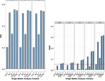
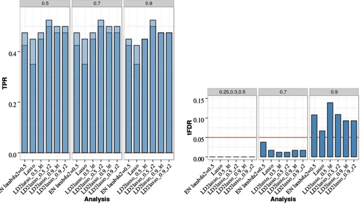
Figure 1 Single-marker analysis (SMA) of chromosome 21 data with two iso-lated QTL, 200 replicates, and sample sizeN= 201. Empirical power is shown [defined as true positive rate (TPR)] on the left: Dark blue represents TPR1 as defined in the main text (TPR including only the significant QTL), and light blue represents TPR2 (TPR also including sig-nificant SNPs linked to QTL at absolute correlation threshold 0.5, 0.7, or 0.9). Empirical thresholded false discovery rate (tFDR) with absolute correlation thresholds 0.25, 0.3, 0.5, 0.7, and 0.9 is shown on the right: Red horizontal line represents the tFDR value of 0.05. GWT, genome-wide threshold that rep-resents the P-value threshold 5.5 3
1028; BH, Benjamini–Hochberg; BY,
this method on the single chromosome 21 simulation with eight true QTL, where it produced a very high number of false positives (irrespective of whether the alternative com-ponent wasfitted with a mixture or a single normal distri-bution), and hence we did not further pursue the PLIS method.
Penalized regression: For PR with FDR control, we also
compared separate and pooled analyses. For the pooled analysis, the SNPs from all three chromosomes were fitted jointly with the Lasso penalty, and the penalty parameter value was chosen based on controlling the FDR at level 0.05. For the separate analysis, the Lasso analysis was performed separately for each chromosome by omitting the SNPs on the other chromosomes and choosing a separate penalty parameter value to control the FDR at level 0.05 for each chromosome.
Comparison among methods
We define a causal true positive (CTP) as a QTL (defined earlier as a functional or causal SNP affecting the pheno-type) that is significant (significant means identified by any of the methods considered). We define a linked true positive (LTP) as a SNP that is significant and has an absolute correlation with a QTL above a certain threshold (T) (note thatTis a threshold on the absolute correlation coefficient,
not the squared coefficient). We define a CLTP as being either a CTP or an LTP. Methods are compared, across the re-plicate simulations, based on (1) true positive rate (TPR) 1 = number of CTPs/number of QTL, (2) TPR2 = number of QTL detected by at least one CLTP (CTP or LTP)/number
of QTL, and (3) threshold-specific empirical tFDR = number of significant SNPs that are not a CLTP at a givenT/number of significant SNPs. For criterion 2, we usedT= 0.9, 0.7, and 0.5 for an increasingly relaxed definition of TP. For criterion 3, we usedT= 0.5, 0.3, and 0.25. Thefirst value (T= 0.5) was chosen because our simulation was designed such that a QTL had a power of 0.5 to be detected and computed using Quanto for a given heritability, sample size, and chro-mosome-wide P-value threshold, and this power decreased to,0.01 for a SNP correlated with the QTL at 0.5 (assum-ing that SNP and QTL have the same allele frequency). The second value (T= 0.3) is just below the threshold of“useful LD”(r= 0.316 orr2= 0.1) as defined by Kruglyak (1999)
and Pritchard and Przeworski (2001) as the value at which the sample size is increased at most 10-fold. The last value (T= 0.25) is close to the threshold used in a previous com-parison study (Ayers and Cordell 2010). For completeness, we also provide tFDR values at the remaining thresholds used for TPR2 (0.9, 0.7).
It is not straightforward to evaluate the empirical FDR in GWAS simulations due to LD. We experimented with alternative ways of defining the tFDR, such as partitioning a chromosome into 100-kb windows and computing tFDR (for a given T) as the number of windows in which the significant SNPs are all false positives divided by the number of windows that contain at least one significant SNP. Such an alternative approach did not change any results signifi-cantly, so we report tFDR for thefirst definition.
The results are presented infigures while more detailed results in the form of tables are available in File S1; the tables include standard errors for all average (across
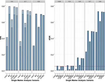
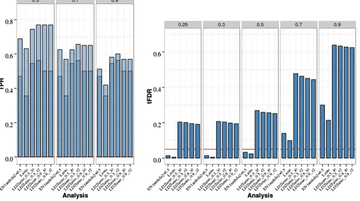
Figure 2 Single-marker analysis (SMA) of chromosome 21 data with eight QTL, 200 replicates, and sample size
N= 201. Empirical power [defined as true positive rate (TPR)] is on the left: Dark blue represents TPR1 as defined in the main text (TPR including only the signif-icant QTL), and light blue represents TPR2 (TPR also including significant SNPs linked to QTL at absolute correlation threshold 0.5, 0.7, or 0.9). Empirical thresholded false discovery rate (tFDR) with absolute correlation thresholds 0.25, 0.3, 0.5, 0.7, and 0.9 is shown on the right: Red horizontal line repre-sents the tFDR value of 0.05. GWT, ge-nome-wide threshold that represents the P-value threshold 5.531028; BH,
replicates) tFDR, TPR1, and TPR2 values that were used for computingP-values for differences in these values between methods or for a one-sided test of average tFDR to exceed level 0.05.
Results and Discussion
Single-chromosome simulation with two or eight QTL: Single-marker analysis
For two isolated QTL, SMA results are summarized in Figure 1 (and Table S1 in File S1). For SMA with GWER control [referred to as genome-wide threshold (GWT) in Figure 1] that controlled the FWER conservatively, the TPR was low (0.2) as expected. For SMA with FDR control, BH and BY controlled the FDR at level 0.05 based on two (three) of the three empirical threshold-specific FDRs (tFDRs), while the local FDR-based approximate oracle procedures LFDR1 and LFDR2 had tFDR values all.0.05 although not significantly
(at nominalP-value of 0.05). The TPR was somewhat higher (0.31) for BY compared with the GWT, while it was sub-stantially higher for BH, LFDR1, and LFDR2 (.0.5).
For the eight-QTL scenario (Figure 2 andTable S2inFile S1), TPR was increased for the FDR-based SMA methods relative to the two-QTL case ($ 0.7 for BH, LFDR1, and LFDR2; 0.6 for BY compared with# 0.4 for GWT). All FDR methods controlled the FDR in the sense of producing at least one tFDR value that was not significantly . 0.05 (nominalP-value). The smallestP-value for exceeding level 0.05 by a tFDR value atT= 0.3 wasP= 0.034 for SMA-BH.
Single-chromosome simulation with two isolated QTL: PR with FDR control
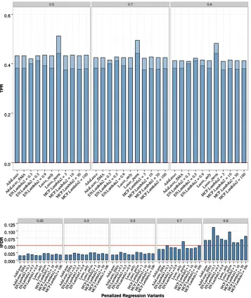
We verified the expectation that Lasso with standard tuning parameter value selection based on CV produces an un-acceptably high empirical FDR (.0.5; results not shown). The results for PR with FDR control for this scenario are presented in Figure 3 andTable S3andTable S4inFile S1.
Figure 3 Penalized regression (PR) anal-yses of chromosome 21 data with two isolated QTL, 200 replicates, and sample sizeN= 201. Empirical power [defined as true positive rate (TPR)] is shown on the top: Dark blue represents TPR1 as defined in the main text (TPR including only the significant QTL), and light blue represents TPR2 (TPR also including sig-nificant SNPs linked to QTL at absolute correlation threshold 0.5, 0.7, or 0.9). Empirical thresholded false discovery rate (tFDR) with absolute correlation thresholds 0.25, 0.3, 0.5, 0.7, and 0.9 is shown on the bottom: Red horizontal line represents the tFDR value of 0.05. The following penalized regression methods (in the order shown) are rep-resented: AdaLasso, adaptive Lasso where all three initial estimators (SMA, Lasso with CV, and ridge regression with CV) produced the same result; EN_Lambda2 =x, elastic net with Lasso portion of l2 = x (x = 0.3, 0.5, 0.9);
Lasso_anly, Lasso with analytical FDR control; Lasso_perm, Lasso with per-mutation FDR control; MCP_lambda2 =
x, minimax concave penalty withl2=x
Differences in empirical tFDR and TPR among all PR methods with analytic FDR control were small; there was a very slight advantage for the elastic net with the mixing parameter set to 0.5 (EN50); Lasso and MCP with different values for the second tuning parameter (from l2 = 3 to
l2= 100) produced almost identical results. All PR methods
were able to control the FDR by producing tFDR values
, 0.05 for all T # 0.5. In terms of power and using the EN50 to represent PR, in comparison with SMA-BH, the average TPR1 and TPR2 values of EN50 were lower with
P-values for the differences ranging from 0.004 to 0.013. Comparing the EN50 with SMA-BY, the average TPR1and TPR2 values of EN50 were higher with allP-values0.002. The Lasso with permutation FDR control had slightly higher tFDR values compared with the Lasso with analytic FDR control; TPR1 and TPR2 of the permutation Lasso were sim-ilar to those of SMA-BH and higher than those of the Lasso with analytic FDR control (smallest P-value for the differ-ence = 0.01). The results for Lasso with permutation FDR
were stable across different sets of permutations (100–400 permutations).
Single-chromosome simulation with eight QTL: PR with FDR control
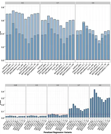
The results for this scenario are presented in Figure 4 and
Table S5andTable S6inFile S1. All PR methods were able to control the FDR by producing tFDR values below (or not significantly above) 0.05 for allT#0.5. Most of the differ-ences in empirical tFDR and TPR among different PR meth-ods with analytic FDR control remained small but some were more pronounced for the eight-QTL data relative to the two-QTL data: EN50 had a higher TRP1 and TRP2 than the Lasso, with aP-value of 231025for the difference in
TPR1 and P= 0.001 for TPR2 at T= 0.9; MCP with low values for the second tuning parameter (l2 = 3, 10) had
lower TPR1 (P-values 1.3310214and 0.003, respectively)
and TPR2 (P-values from 2310215to 0.03 and from 0.003
to 0.33, respectively, with the upper end of each range
Figure 4 Penalized regression (PR) anal-yses of chromosome 21 data with eight QTL, 200 replicates, and sample size
N= 201. Empirical power [defined as true positive rate (TPR)] is shown on the top: Dark blue represents TPR1 as de-fined in the main text (TPR including only the significant QTL), and light blue represents TPR2 (TPR also including sig-nificant SNPs linked to QTL at absolute correlation threshold 0.5, 0.7, or 0.9). Empirical thresholded false discovery rate (tFDR) with absolute correlation thresholds 0.25, 0.3, 0.5, 0.7, and 0.9 is shown on the bottom: Red horizontal line represents the tFDR value of 0.05. The following penalized regression meth-ods (in the order shown) are represented: AdaLasso, adaptive Lasso where all three initial estimators (SMA, Lasso with CV, and ridge regression with CV) produced the same result; EN_Lambda2 =x, elastic net with Lasso portion ofl2=x(x= 0.3,
0.5, 0.9); Lasso_anly, Lasso with analytical FDR control; Lasso_perm, Lasso with per-mutation FDR control; MCP_lambda2 =x, minimax concave penalty with l2=x
representing TPR2 atT= 0.5) than the Lasso. Power was expectedly higher relative to the two-QTL scenario (for EN50, TPR2 atT= 0.5 increased from 0.43 to 0.73). Com-paring the EN50 with SMA-BH, the average TPR1 and TPR2 values of EN50 were lower with P-values for the differences ranging from 5 3 10222to 0.001. Comparing
the EN50 with SMA-BY, EN50 had a significantly higher value for TPR2 atT= 0.5 (P-value 0.0005) while EN50 had a lower value for TPR1 (P-value 0.005). In general, differ-ences among PR methods were largest for TPR1 and TPR2 at T = 0.9 and were diminished for TPR2 with T = 0.5. Comparing Lasso with permutation vs.analytic FDR esti-mation, the permutation Lasso had lower TPR1 and TPR2 withP-values for the differences#0.0006. It is surprising that the permutation method, which was the most power-ful approach in the two-QTL scenario, is so conservative in the eight-QTL scenario. This appears to be due to the fact that permuting the phenotypes, while justified under the global null hypothesis of no association between any SNPs and the phenotypes, is conservative when evaluating the significance of a QTL in the presence of substantial signal from other QTL. By permuting the phenotype, which con-sists of both fixed signal and random error, the contribu-tion of the random errors is overestimated. This does not affect the validity of the permutation approach in terms of properly controlling the FDR but does diminish power in cases like the eight-QTL scenario.
The eight-QTL simulation included two groups of two QTL each with within-groupr20.5 (absolute correlation among
SNP doses of 0.71). Because of the Lasso’s tendency to select only a single SNP per group and the EN’s ability to deal with colinearity and potential coselection of correlated SNPs (SNPs in LD), we took a closer look at the behavior of Lasso and EN in this situation. Averaged over both groups and the 200 replicate simulations and including LTPs (T= 0.5), the Lasso
selected zero SNPs in 22%, one SNP in 43%, two SNPs in 26%, and more than two SNPs in 9% of cases. By comparison, the EN selected zero SNPs in 19%, one SNP in 37%, two SNPs in 31%, and more than two SNPs in 13% of cases. Expectedly the EN selected two and more than two SNPs more frequently but the difference was not substantial.
Single-chromosome simulation with two/eight QTL: Fusion-type penalties
Here we focused on the LD2lasso withf(the relative weight given to the Lasso penalty)fixed at two different values (0.9, 0.5), with the two LD functionsh(r) = |r| andh(r) =r2, and
with h(r) = 0 if |r| ,0.85 [for this threshold, the median number of SNP “neighbors” was 2 with interquartile range (IQR) 0–5 and range 0–39] or |r|,0.50 (median number of SNP neighbors = 14 with IQR 6–25 and range 0–102). Be-cause we did not optimize the implementation of the LD2lasso for computational speed, we compared the LD2lasso with the Lasso and EN50 based on only 20 data replicates that were randomly selected from the 200 replicates. For the chromosome 21 data with two isolated QTL, the LD2lasso achieved higher power than Lasso and EN50 while maintain-ing FDR control (Figure 5 and Table S7 in File S1). The largest difference was the increase in TPR1 from 0.35 for the Lasso to 0.5 for the best LD2lasso analysis withf = 0.5 andh(r) =r2(P-value,0.05), while all other differences in
TPR1 and TPR2 were smaller.
For the chromosome 21 data with eight QTL (Figure 6 and Table S8 in File S1), however, all LD2lasso variants were unable to control the FDR with average tFDR values at the lowest threshold ofT= 0.25 near 0.2 (P-value for the differences to FDR level 0.05 ,431024). We recall that
the eight-QTL data contained a group of four QTL with weak pairwise LD (0.01#r2#0.1); the high tFDR values (0.2–
0.26) for LD2lasso were mostly due to SNPs in LD with the
Figure 5 Empirical power [true positive rate (TPR)] and thresholded false discov-ery rate (tFDR) for LD2lassovs.Lasso and elastic net (EN) penalized regression (PR) analyses of chromosome 21 data with two isolated QTL, 20 randomly selected replicates, and sample size N = 201. Dark blue represents TPR1 as defined in the main text (TPR including only the significant QTL), and light blue repre-sents TPR2 (TPR also including signifi -cant SNPs linked to QTL at absolute correlation threshold 0.5, 0.7, or 0.9). The empirical tFDR was computed atfive absolute correlation thresholds between causal and linked SNPs (T= 0.25, 0.3, 0.5, 0.7, 0.9). The red horizontal line represents the tFDR value of 0.05. EN_Lambda2 = 0.5 denotes the elastic net with Lasso portion of l2 = 0.5;
LD2lasso_0.9_r2 (LD2lasso_0.9_|r|)
rep-resents the LD2lasso with weight on the Lasso penalty equal tof= 0.9 and LD functionh(r) =r2(h(r) = |r|). The LD function was set to zero when the
group of four causal SNPs at small absolute correlation val-ues. In terms of TPR, the difference in TPR1 between the best LD2lasso analysis withf= 0.5,h(r) =r2, and |r|,0.85
(|r| , 0.50) and the Lasso had a P-value of 5.4 3 1025
(1.731025), while the difference in TPR1 between the best
LD2lasso and the EN50 had a largerP-value of 0.10 (0.008). TPR2 values were also higher, but mostP-values for the dif-ferences in TPR2 between the same methods were . 0.05 due to smaller differences (less than half) and the small number of replicates.
Single-chromosome simulation with eight QTL: PR vs. SMA and CAR
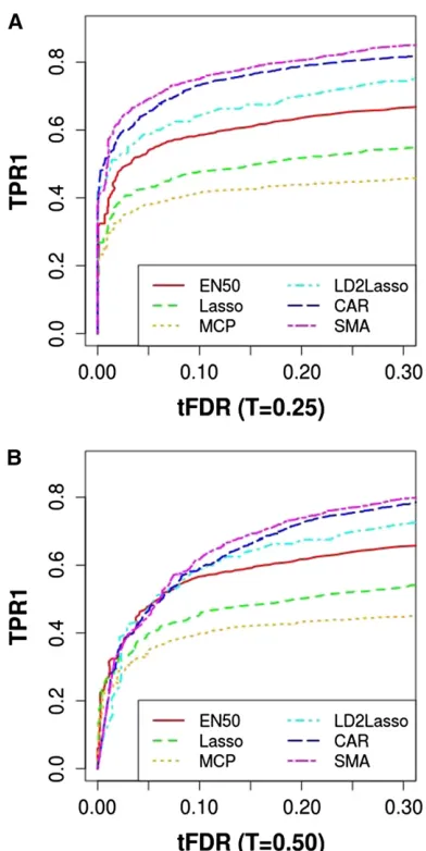
Because all previous comparisons focused on differences among methods in empirical TPR and tFDR for a single FDR cutoff of 0.05, here we present TPR1 vs.tFDR atT= 0.25 and T= 0.50 (Figure 7) and TPR2 (T= 0.50)vs.tFDR at
T= 0.25 and T = 0.50 (Figure 8). Figure 7 and Figure 8 were generated by varying theP-value cutoff for SMA and CAR and varying the penalty parameter for PR. In terms of power to detect causal SNPs (TPR1) and when using the most re-laxed definition of tFDR (withT= 0.25), SMA dominated all other methods with CAR being second followed by LD2lassso and EN50, with Lasso and MCP (l2= 10) performing worst
(Figure 7). When using a more stringent definition of false positives with tFDR at T = 0.50, SMA/CAR dominated in terms of TPR1 only for tFDR values.0.05.
In terms of power to detect QTL with causal or linked SNPs (TPR2 atT= 0.5) (Figure 8) and when using the most relaxed definition of tFDR (withT= 0.25), EN50 and SMA (the latter for higher tFDR (T= 0.25) values) slightly dom-inated the other methods, with the LD2lasso now perform-ing worst for the most relevant range of tFDR (T = 0.25) from 0.01 to 0.10. When replacing tFDR (T = 0.25) with
tFDR (T= 0.50), EN50 performed best (slightly better than Lasso and MCP), with SMA, CAR, and LD2lasso now sepa-rated as the worst performers.
Single-chromosome simulation with two/eight QTL: Previous approaches
The multisplit analysis of Meinshausen et al. (2009) was evaluated based on a random subset of 20 replicates of the chromosome 21 two-QTL data and on another random subset of 20 replicates of the chromosome 21 eight-QTL data (Table S9inFile S1). It controlled the FDR quite con-servatively (all tFDR values equal to zero) and had low power relative to the single-step PR methods with FDR con-trol, as expected. Power (TPR) was,0.18 for the two-QTL data and , 0.21 for the eight-QTL data. P-values for the differences in TPR between the multisplit analysis and the Lasso ranged from 0.01 to 0.04 for the two-QTL data and from 2.431027to 431024for the eight-QTL data.
The adaptive Lasso with local FDR control of Sampson
et al. (2013) was evaluated using all 200 replicates of the chromosome 21 two-QTL and eight-QTL data (Table S10in
File S1). R code for executing this method was generously provided to us by thefirst author (H. Yi). For our data, the local FDR adaptive Lasso controlled the FDR at the local FDR threshold of 0.1 (tFDR values ,0.05), but its power (TPR) was much lower than that of the Lasso for both the two-QTL and the eight-QTL data (P-values for the differen-ces in TPR to the Lasso ranged from 1310212to 2310213
and from 2.4310267to 2.5310283, respectively). When
raising the local FDR threshold to 0.5, the FDR was not controlled for the two-QTL data (tFDR values highly signif-icantly .0.05) but was controlled for the eight-QTL data (tFDR values , 0.05) where the TPR values, however, remained significantly below the values of the Lasso.
Figure 6 Empirical power [true posi-tive rate (TPR)] and thresholded false discovery rate (tFDR) for LD2lassovs.
Lasso and elastic net (EN) penalized regression (PR) analyses of chromo-some 21 data with eight QTL, 20 ran-domly selected replicates, and sample size N = 201. Dark blue represents TPR1 as defined in the main text (TPR including only the significant QTL), and light blue represents TPR2 (TPR also including significant SNPs linked to QTL at absolute correlation thresh-old 0.5, 0.7, or 0.9). The empirical tFDR was computed at five absolute correlation thresholds between causal and linked SNPs (T = 0.25, 0.3, 0.5, 0.7, 0.9). The red horizontal line rep-resents the tFDR value of 0.05. EN_Lambda2 = 0.5 denotes the elas-tic net with Lasso portion ofl2= 0.5;
LD2lasso_0.9_r2(LD2lasso_0.9_|r|)
rep-resents the LD2lasso with weight on the Lasso penalty equal tof= 0.9 and LD functionh(r) =r2(h(r) = |r|). The LD function was set to zero when the
PUMA was run on the eight-QTL data with 200 replicates, choosing the 2D-MCP method, omitting the SNP preselection step and otherwise using default parameter values. The results are inTable S11inFile S1for four differentP-value thresholds for SNP selection ranging from 1 31027to 0.05, and these
results need to be compared with our MCP with analytic FDR control [and fourfixed values of the second tuning parameter
l2 in (9)] in Table S6. The authors (Hoffman et al. 2013)
recommended aP-value threshold of 131027for 2D-MCP,
which controlled the FDR in terms of the tFDR values inTable S11; the next lower threshold of 1 31026had tFDR values .0.06 whose one-sided test for exceeding level 0.05 had
P-values from 0.055 to 0.11. Overall, TPR1 and TPR2 values for 2D-MCP were significantly below those for MCP with an-alytic FDR control (P-values for differences from 931025to
8310229for 2D-MCP SNP selection threshold 131027and
from 0.032 to 2310222for 2D-MCP SNP selection threshold
1 3 1026). To explain these differences, we looked at the
values for l2 for the models chosen in PUMA by AIC over
the 200 data sets, which surprisingly had a median of 3.46, with almost all values well below 10. For our own MCP anal-ysis with FDR control we had chosen four values for the sec-ond tuning parameter (3, 10, 30, and 100), of which the lowest value performed the worst. We then replaced the heu-ristic AIC model selection followed by SNP selection of PUMA with our analytic FDR tuning parameter selection, which sig-nificantly improved TPR1 and TPR2 (last column of Table S11). The analytic FDR criterion selected models with larger values forl2with a median of 33.6 (as well as larger values
forl1, median 0.166vs.0.310) This improvement still
under-performed the results inTable S6 because PUMA uses a (in-ternally determined) grid of values forl1andl2in 2D-MCP,
which was too sparse for optimal performance of the analytic FDR approach.
Figure 8 Plot of true positive rate TPR2vs.thresholded false discovery rate (tFDR): TPR2 (T= 0.50)vs.tFDR (T= 0.25) and TPR2 (T= 0.50)vs.
tFDR (T= 0.50). TPR2 and tFDR are defined in the main text. MCP was run withl2= 10. CAR represents correlation-adjusted marginal correlations.
Figure 7 Plot of true positive rate TPR1vs.thresholded false discovery rate (tFDR): TPR1vs.tFDR (T= 0.25) and TPR1vs.tFDR (T= 0.50). TPR1 and tFDR are defined in the main text. MCP was run withl2= 10. CAR
Analyses of multiple chromosomes
Here we analyzed the simulated data including chromo-somes 19 (no QTL), 21 (eight QTL), and 22 (two QTL) with 200 replicates. For SMA, the average tFDR values for pooled and separate BH analyses and for the local FDR grouping procedure were all .0.05 forT = 0.25 and 0.3 but most were insignificantly higher (largestP-value of 0.001 for sep-arate BH). Differences in TPR between SMA-based pooled and separate analyses and the grouping procedure of Cai and Sun (2009) were small and insignificant, although there was a trend for increasing TPR from pooled analysis to sep-arate analysis to the grouping procedure (see Table S12in
File S1).
For penalized regression using Lasso PR with analytic FDR control, pooled and separate analyses controlled the FDR in terms of their average tFDR values, and differences in TPR between the pooled and the separate Lasso were small and insignificant (Table S13inFile S1). We therefore compared the separate and pooled analyses for individual chromosomes. FromTable S13, we can see that for chromo-some 21 (with eight QTL), TPR1 and TPR2 decreased chromo- some-what from separate to pooled analysis withP-values for the differences ranging from 0.02 to 0.05. For chromosome 22 (with only two QTL), in contrast, TPR1 and TPR2 increased significantly as expected from separate to pooled analysis with allP-values,4310210.
Analysis of real data
We applied PR and SMA methods to data from the Health ABC GWAS of interleukin 6 soluble receptor (IL-6 SR). The analysis included 786 Health ABC Caucasians who had both GWAS and serum IL-6 SR measurements (a continuous phenotype, approximately normally distributed) avail-able (see File S2for details). The genotype data included 750,424 SNPs (after standard edits) from chromosomes 1, 3, 4, 6, and 19. Covariates included in the analysis models were age, gender, site of data collection, and one principal component score obtained using Eigenstrat. We analyzed
these data by SMA with GWER threshold (SMA-GWT), by SMA with BH FDR control (SMA-BH), and with the elastic net with 50% Lasso penalty (EN50) and analytic FDR con-trol. SMA-GWT is commonly used in practice, and SMA-BH performed best among all SMA methods with FDR control on the simulated data. The elastic net was chosen as the single PR method because it performed best on the simulated data among all PR methods combined with our novel method for FDR control and because differences among PR methods were generally small. For SMA-BH and EN50 (EN50-sep), chromo-somes were analyzed separately, and for EN50, a joint anal-ysis of all chromosomes was also performed (EN50-joint).
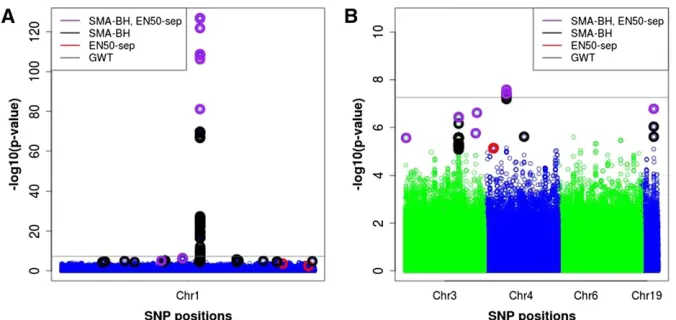
Chromosome 1 represents a special situation in that it contains a region with an extremely strong QTL signal. The very stringent SMA-GWT threshold identified 74 SNPs for this chromosome, many more than the 15 EN50-sep SNPs (see Table 1). Of these 74 SNPs, 61 were in LD above the absolute correlation threshold of 0.25 with EN50-sep SNPs, and the remaining 13 SNPs had largest absolute correlations with EN50-sep SNPs between 0.20 and 0.24 and therefore likely still overlap with EN50-sep SNPs (given the very strong sig-nal) rather than represent independent signals. The EN50-sep selected a small subset of the peak area SNPs that had the smallest SMAP-values (Figure 9). While the SMA-GWT SNPs were all located in the area of the major peak, several EN50-sep SNPs were located in regions clearly EN50-separated from the peak, which mostly overlapped with SNPs detected by SMA-BH except for one EN50-sep SNP (see Figure 9). Expectedly, SMA-BH identified the largest number of SNPs (161), of which 101 were in LD above the absolute correlation thresh-old of 0.25 with EN50-sep SNPs. The remaining 60 SMA-BH SNPs had largest absolute correlations with EN50-sep SNPs between 0.07 and 0.24, indicating together with Figure 9 that SMA-BH selected some SNPs physically well separated from and likely not in LD with any EN50 SNPs. To check on the interpretation of the SNP–SNP correlation values, we simulated independent SNPs forN= 786 representing 11 different MAF values between 0.01 and 0.5 (assuming Hardy–Weinberg
Table 1 Analysis of the real data with single-marker analysis, using the genome-wide thresholdP-value<5.5 310-8(SMA-GWT) or Benjamini–Hochberg FDR control (SMA-BH) applied separately to the data on each chromosome and elastic net penalized regression with analytic FDR control applied separately to each chromosome (EN50s) or jointly across allfive chromosomes (EN50j)
Analysis Method Significant SNPs
Chromosome
1 3 4 6 19
SMA-GWT No. sig 74 0 8 0 0
\EN50s 9/17/42/61 0/0/0/0 6/8/8/8 0/0/0/0 0/0/0/0
SMA-BH No. sig 161 30 10 0 3
\EN50s 13/23/49/101 5/30/30/30 6/9/9/9 0/0/0/0 1/1/3/3
EN50j No. sig 14 3 3 0 0
\EN50s 14/14/14/14 2/2/2/2 2/2/2/2 0/0/0/0 0/0/0/0
EN50s No. sig 15 5 8 0 1
\SMA-GWT 9/9/9/9 0/0/0/0 6/6/6/6 0/0/0/0 0/0/0/0
\SMA-BH 13/13/13/14 5/5/5/5 6/6/6/6 0/0/0/0 1/1/1/1
equilibrium) and computed all pairwise absolute correlations over 100,000 replications, yielding 75th, 95th, and 99th per-centiles just below 0.025, 0.07, and 0.13, respectively, with a maximum value of 0.31. Based on our simulation studies (in particular the eight-QTL simulation), SMA-BH may have higher power than EN50-sep (by 10%) but also may not completely control the FDR, so the 60 SMA-BH SNPs with very small correlations to EN50-sep SNPs may represent some ad-ditional true signals and some false positives. We also reran EN50-sep on chromosome 1 by excluding all peak area SNPs but including a single peak area SNP (with the smallest P -value) in the model without shrinkage, but this analysis did not identify any additional SNPs (such as any of the 60 SMA-BH SNPs) compared to the previous EN50-sep analysis.
On chromosome 4, SMA-GWT, SMA-BH, and EN50-sep identified similar numbers of SNPs, 8 for SMA-GWT (all correlated with EN50 SNPs), 10 for SMA-BH (all but 1 correlated with EN50 SNPs), and 8 for EN50 (6 of which were correlated with SMA-GWT or SMA-BH SNPs).
On chromosomes 3 and 19, no QTL were identified with the stringent SMA-GWT, while SMA-BH and EN50-sep identified the same QTL (Table 1 and Figure 9). For chromo-some 3, the 30 SMA-BH SNPs were all in LD (absolute cor-relation threshold of 0.25) with the 5 EN50-sep SNPs, and for chromosome 19, the 3 SMA-BH SNPs were all in LD with the 1 EN50-sep SNP. No SNPs were identified by any method on chromosome 6. Overall, these results show that SMA-BH and EN50-sep identify very similar candidate regions in a genome scan; that EN50 (and other PR methods) will select a subset of SNPs in a cluster of correlated SNPs, here those with the smallest SMAP-values; and that for follow-up (fine-mapping)
studies, all EN50 (or other PR) identified SNPs plus a set of SNPs correlated with the identified SNPs (above a certain threshold) should be considered.
Finally, the joint analysis of all chromosomes by EN50 with FDR control (EN50-joint), compared to the separated analyses (EN50-sep), identified fewer SNPs (20 SNPs for joint compared with 29 SNPs for sep). EN50-joint identified one SNP on chromosome 3 and another on chromosome 4 that were not in LD with EN50-sep SNPs. The
EN50-joint SNP on chromosome 3 is likely a false positive due to its2log10(P-value) being much smaller than those of
all other identified (by any method) SNPs (Figure 10). The EN50-joint SNP on chromosome 4, however, was in LD (ab-solute correlation.0.9) with a SMA-BH SNP.
Concluding remarks
The goals of this study were to provide a review and an independent comparison of penalized regression methods with single-marker analysis for variable (SNP) selection in GWAS and to implement and evaluate penalty/tuning param-eter value selection by FDR control. A recent application of PR to GWAS (Waldmannet al.2013, p. 1) arrived at this conclu-sion:“Hence, we can conclude that it is important to analyze GWAS data with both the lasso and the elastic net and an alternative tuning criterion to minimum MSE is needed for vari-able selection.”Here we provided such an alternative criterion. We provided both a simple, approximate analytic method and a permutation-based method for FDR control in PR. The analytic method performed consistently well although being somewhat conservative. The permutation method expectedly had higher power (was less conservative) than the analytic method in the two-QTL scenario but was more conservative than the analytic method in the eight-QTL scenario. This initially unexpected behavior of the permutation method appears to be due to the fact that permuting the phenotypes means permuting some signal along with the random error and thus overestimates the amount of random error in the data. This causes the permutation method to become in-creasingly conservative with increasing numbers and effect sizes of causal SNPs (QTL). Because our simulated data had small sample sizes (200) and contained QTL jointly explain-ing 20 or 48% of the phenotypic variance (for the two- or eight-QTL data, respectively), this problem of the permuta-tion method is more pronounced in our simulapermuta-tion than in real GWAS data characterized by very large sample sizes (thousands to tens of thousands) and small SNP effects (explaining # 1% of the overall variation). However, the problem may manifest itself also in real data, when there are larger numbers of causal SNPs or causal SNPs with larger
Figure 9 Plot of –log10(P-value) for SNPs on
chromosomes 1 (left), 3, 4, 6, and 19 (right) for the real data. The purple, black, and red circles represent significant SNPs selected by both SMA with BH FDR control (SMA-BH) and EN50 (elastic net with 50% weight on L1), by SMA-BH only, and by EN50 only, respec-tively. EN50-sep denotes EN50 applied to each chromosome separately. The gray line is the genome-wide threshold of 5.531028, above
effect sizes as in our Health ABC GWAS. This is unfortunate because the main advantage of multimarker over single-marker approaches is that they are able to use the signal from other markers in determining significance. It may be possible to overcome this limitation by estimating the residuals using thefitted model and then permuting the residuals instead of the phenotype; we are currently investigating the perfor-mance of this approach.
Based on our comparisons with previous strategies for SNP selection in PR, it appears that our analytic FDR criterion is currently the best approach to SNP selection when using PR for GWAS, and this approach should be appealing to practi-tioners who desire a measure of error, in particular in terms of FDR, associated with the selected SNPs. Finally we note that our simple analytic FDR method can also be applied to pe-nalized logistic regression.
When the focus is on variable selection (here the identification of a causal SNP by itself or a linked SNP) and not on estimation or prediction, our results indicate that among all PR methods investigated here, a version of the elastic net (EN50) performs better than the other PR methods in most situations, although differences were often small. Based on our analyses of simulated and real data, the EN50 should identify QTL regions that are very similar to those identified by SMA combined with BH FDR control. In contrast with SMA-BH, EN50 identifies a QTL region with a single SNP or few SNPs, and hence subsequent fine-mapping should include the EN50 SNPs plus additional SNPs in LD with the EN50 SNPs above a certain threshold. Expectedly, EN50 and SMA-BH have substantially more power than SMA with the genome-wide type-I error threshold.
Incorporating fusion-type penalties developed for covari-ates measured on graphs may improve power but can also generate more false positives or rather wide QTL regions for follow-up, in situations when there are multiple, moderately correlated causal SNPs located on the same chromosome and false positives are defined as any significant SNPs correlated with a causal SNP below an absolute value of 0.25.
When applying PR to large genome-wide data sets for joint (pooled) analysis of all chromosomes, prescreening SNPs based on SMA P-values is still necessary due to the high memory requirements for holding the entire SNP genotype
matrix in memory (see Hoffmanet al.2013 for more details). We note that if prescreening is performed, then for tuning parameter value selection by our analytic FDR method the number of markers (p) in (13) should be set to the total number of markers (prior to preselection) to maintain control of the FDR (which should produce the same result as what would be obtained without preselection). It would, however, be prudent to perform PR with FDR control both on the entire set of SNPs from all chromosomes (pooled analysis) and sep-arately on each chromosome (separate analysis). Our results from the simulated and real data representing several chro-mosomes indicate that the pooled analysis does not necessar-ily provide better power for all chromosomes.
We note that currently there is substantial interest in extending GWAS of single phenotypes to high-dimensional phenotypes (e.g., Marttinen et al. 2012). While high-dimensional phenotypes allow aspects of modeling that are not feasible with a single phenotype, the results of the current study still provide useful information for the design of anal-ysis methods for GWAS of high-dimensional phenotypes.
Finally, code used for data simulation and code for EN50 analysis with analytic FDR control are provided in File S3. An example simulated data set with eight QTL on chromo-some 21 is available at the Dryad Digital Repository (http:// doi.org/10.5061/dryad.hc445).
Acknowledgments
This work was supported by the National Institute of General Medical Sciences grant R01HG005254 (to I.H.), by the National Institute on Aging grant 1R01AG032098-01A1 and the National Heart, Lung, and Blood Institute grant R01HL101250 (to Y.L.), and by a Virginia Tech Genetics, Bioinformatics, and Computational Biology Ph.D. program fellowship (to H.Y.). The Health ABC study was supported by the National Institute on Aging contracts N01AG62101, N01AG62103, and N01AG62106. Genotyping services were provided by the Center for Inherited Disease Research (CIDR). CIDR is fully funded through a federal contract from the National Institutes of Health to The Johns Hopkins University, contract HHSN268200782096C.
Figure 10 Plot of2log10(P-value) for SNPs on