Estimating the Number of Subpopulations (K) in Structured Populations

| INVESTIGATION

Estimating the Number of Subpopulations (

K

) in

Structured Populations

Robert Verity*,1_{and Richard A. Nichols}† *Medical Research Council Centre for Outbreak Analysis and Modelling, Imperial College London, London W2 1PG, United Kingdom, and†Queen Mary University of London, London E1 4NS, United Kingdom ORCID ID: 0000-0002-4801-9312 (R.A.N.).

ABSTRACTA key quantity in the analysis of structured populations is the parameterK, which describes the number of subpopulations that make up the total population. Inference ofKideally proceeds via themodel evidence, which is equivalent to the likelihood of the model. However, the evidence in favor of a particular value ofKcannot usually be computed exactly, and instead programs such as Structure make use of heuristic estimators to approximate this quantity. We show—using simulated data sets small enough that the true evidence can be computed exactly—that these heuristics often fail to estimate the true evidence and that this can lead to incorrect conclusions aboutK. Our proposed solution is to use thermodynamic integration (TI) to estimate the model evidence. After outlining the TI methodology we demonstrate the effectiveness of this approach, using a range of simulated data sets. Wefind that TI can be used to obtain estimates of the model evidence that are more accurate and precise than those based on heuristics. Furthermore, estimates ofKbased on these values are found to be more reliable than those based on a suite of model comparison statistics. Finally, we test our solution in a reanalysis of a white-footed mouse data set. The TI methodology is implemented for models both with and without admixture in the software MavericK1.0.

KEYWORDSpopulation structure;K; model evidence; thermodynamic integration; model comparison

T

HE detection and characterization of population structure is one of the cornerstones of modern population genetics. Ever since Wright (1949) and his contemporaries (Malécot 1948) it has been recognized that genetic samples obtained from a large population may be better understood as a series of draws from multiple partially isolated subpopulations or demes. While traditional methods (such as those based on thefixation index,FST) assume that the allocation of individ-uals to demes is knowna priori, many modern programs such as Structure (Pritchardet al.2000; Falushet al.2003a, 2007; Hubiszet al.2009) take a different approach, attempting to infer the group allocation from the observed data. What makes this possible is the simple genetic mixture modeling framework used by these programs, together with the effi -ciency of Markov chain Monte Carlo (MCMC) methods for sampling from this broad class of models.

However, even within theflexible framework of Bayesian mixture models, the number of demes (denotedK) is difficult to ascertain. While the allocation of individuals to demes is a parameter withina particular model, the value of Kis fixed for a given mixture model, and so the problem of estimating

Kinvolves a comparisonbetweenmodels. One of the most com-mon ways of comparing between models in a Bayesian setting is through the model evidence, defined as the probability of the observed data under the model (equivalently the likelihood of the model). This quantity can be estimated for a range ofK, and the model with the highest evidence value can then become the focus of our analysis. However, there are two potential issues with this approach. Thefirst one is philosophical and revolves around the idea that there is a single true value ofKthat we can estimate from the data. In reality populations are rarely divided into discrete subpopulations, and so the idea of a single true value ofKdoes not strictly apply. This does not mean thatK

cannot be a useful quantity, but it is better viewed as aflexible parameter that describes just one point on a continuously vary-ing scale of population structure. Thisflexible interpretation of

Khas been advocated by a number of previous authors (Raj

et al.2014; Jombart and Collins 2015), including the authors of the Structure program (Pritchardet al.2010).

Copyright © 2016 by the Genetics Society of America doi: 10.1534/genetics.115.180992

Manuscript received July 21, 2015; accepted for publication June 4, 2016; published Early Online June 10, 2016.

Supplemental material is available online atwww.genetics.org/lookup/suppl/doi:10. 1534/genetics.115.180992/-/DC1.

1_{Corresponding author: MRC Centre for Outbreak Analysis and Modelling, Imperial} College London, London W2 1PG, United Kingdom. E-mail: [email protected]

The second issue is purely statistical—computing the model evidence in complex, multidimensional models is not straightforward. For this reason it is common to resort to heuristic estimators of the true evidence. These heuristics tend to have some direct mathematical connection to the model evidence, but also make certain simplifying assump-tions in their derivation. For example, in the original article on which Structure is based, Pritchardet al.(2000) comment on the difficulties in obtaining the model evidence directly and instead opt for anad hoc procedure in which a heu-ristic (denoted LK here) is used as an approximation of

223logðevidenceÞ:The derivation of this statistic rests on certain simplifying assumptions, and the authors are careful to emphasize that these assumptions are“dubious.”

Here we focus on the latter problem: reliable estimation of the model evidence. Rather than resorting to heuristics, what we want is a direct way of estimating the model evidence that is both accurate and straightforward to implement. As noted by Gelman and Meng (1998), such a method already exists and has been known in the physical sciences for some time. This method—referred to in the statistical literature as ther-modynamic integration (TI)—uses the output of several closely related MCMC chains to obtain a direct estimate of the evidence. Crucially, this is not just another heuristic. Rather, it is a true statistical estimator that can be evaluated to an arbitrary degree of precision by simply increasing the number of MCMC iterations used in the calculation. The TI methodology was introduced into population genetics by Lartillot and Philippe (2006) and has since been applied to a range of problems in phylogenetics and coalescent theory, including comparing models of demographics (Baele et al.

2012), migration (Beerli and Palczewski 2010), relaxed mo-lecular clocks (Lepageet al.2007), and sequence evolution (Blanquart and Lartillot 2006).

In the remainder of this article we demonstrate the effec-tiveness of TI as a method for estimatingKin simple genetic mixture models. For small data sets wefind that the TI esti-mator is several orders of magnitude more accurate and pre-cise than theLKestimator for the same computational effort.

We also explore the ability of different statistics to correctly estimateKfor larger data sets,finding that TI outperforms Evanno’sDK (Evannoet al. 2005), the Akaike information criterion (AIC), the Bayesian information criterion (BIC), and the deviance information criterion (DIC). Finally we reanalyze data from an earlier study on the genetic structure of white-footed mouse populations in New York City (Munshi-South and Kharchenko 2010b). All of the methods described here are made available through the program Mav-ericK (www.bobverity.com/MavMav-ericK).

Materials and Methods

Evidence and Bayes factors

In a Bayesian setting the problem of deciding between competing models can be addressed using Bayes’rule. The

posterior probability of the model M;given the observed datax;can be written

PrðMjxÞ ¼PrðxjMÞ PrðMÞ

PrðxÞ : (1)

The quantity PrðxjMÞ—the probability of the observed data x given just the model M—is defined as the model evidence.

The ratio of the evidence between competing models, known as the Bayes factor, can be used to measure the strength of evidence in favor of one model over another. Bayes factors can be used on their own, or they can be com-bined with priors on the different models to arrive at the posterior odds:

PrðM1jxÞ

PrðM2jxÞ

|fflfflfflfflfflfflffl{zfflfflfflfflfflfflffl}

posterior odds ratio

¼ PrðxjM1Þ

PrðxjM2Þ

|fflfflfflfflfflfflffl{zfflfflfflfflfflfflffl}

Bayes factor

 3 PrðM1Þ

PrðM2Þ

|fflfflfflfflffl{zfflfflfflfflffl}

prior odds ratio 

: (2)

A large Bayes factor in (2) provides evidence in favor of model

M1 over modelM2;whereas a small Bayes factor provides evidence in favor of modelM2over modelM1:A useful scale for interpreting Bayes factors can be found in Kass and Raftery (1995); however, it is important to note that this scale is meaningful only if priors are chosen appropriately (seeDiscussion).

The problem of estimating the number of demes in a structured population can be understood in this light: If we letMKdenote a genetic mixture model in whichKdemes

are assumed, then the problem of estimatingKbecomes one of comparing between different models. Ideally we want to solve this problem using the exact model evidence, PrðxjMKÞ:Unfortunately, however, calculating the model

ev-idence in complex, multidimensional models is not straight-forward, as most of the time we cannot write down the probability of the data under the model without also condi-tioning on certain known parameters, denotedu:Obtaining the evidence from the likelihood requires that we integrate over a prior onu:

PrðxjMKÞ ¼

Z

uPrðxju;MKÞ PrðujMKÞ du: (3)

It is this integration step that makes calculating the model evidence difficult in practice. In genetic mixture models u might represent the allele frequencies in allKdemes, perhaps alongside some additional admixture parameters, making the integral in (3) extremely high dimensional (a 100-dimensional integral would not be uncommon). For this rea-son it makes practical sense to turn to numerical methods or heuristic approximations.

Estimating and approximating the evidence

Perhaps the simplest way of estimating the model evidence is through the harmonic mean estimator, h^K (Newton and

Raftery 1994),

PrðxjMKÞ

"

1

t Xt

m¼1

1 Prðxjum;MKÞ

#₂1

¼^hK; (4)

whereum form2 f1;. . .;tgdenotes a series of draws from

the posterior distribution ofu:Part of the appeal of this esti-mator is its simplicity—it is straightforward to calculate^hK

from the output of a single MCMC run. As an example, the program Structurama (Huelsenbeck and Andolfatto 2007; Huelsenbecket al.2011), which contains within it a version of the basic Structure model, has an option for using^hK to

estimate the model evidence (we note that this is not the primary purpose of Structurama, which also implements a Dirichlet process model). However, in spite of its intuitive appeal, the harmonic mean estimator has been widely criti-cized due to its instability; ^hK has been found to be very

sensitive to the choice of prior, often being dominated by the reciprocal of a few small values (Neal 1994; Raftery

et al.2006).

To avoid some of the problems inherent in the harmonic mean estimator, the approach taken by Pritchardet al.(2000) was to define the heuristic estimatorLK(our notation) as

22   logPrðxjMKÞ

m^þs^2

4 ¼LK; (5)

wherem^ and^s2are simple statistics that can be calculated from the posterior draws (see Supplemental Material,File S1 for a more detailed derivation of this and other statistics). The key assumption that underpins this heuristic is that the posterior deviance is approximately normally distributed, which may or may not be true in practice.LKis usually

eval-uated for a range ofK, and the smallestLK(corresponding to

the largest evidence) is used as an indication of the most likely model. Alternatively, these values can be transformed out of log space to provide direct estimates of the evidence that, once normalized, can be used to approximate the full posterior distribution ofK:

PrðMKjxÞ

exp2ð1=2ÞLK

P

kexp

2ð1=2ÞLk

: (6)

This procedure is rarely carried out in practice, despite being recommended in the Structure software documentation (Pritchardet al.2010).

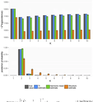
Figure 1 True and estimated val-ues of the model evidence in log space and in linear space. Error bars give 95% confidence inter-vals around estimates.

Thermodynamic integration

The TI estimator differs fundamentally fromLK in the sense

that it is not a heuristic estimator—it makes no simplifying assumptions about the distribution of the likelihood. It also differs from^hK in that it is well behaved, havingfinite and

quantifiable variance. The approach centers around the

“power posterior”(Friel and Pettitt 2008), defined as follows:

P_bðujx;MKÞ ¼Prðxju;MKÞ

b_PrðujM

KÞ uðxjb;MKÞ :

(7)

This is nothing more than the ordinary posterior distribution ofu;but with the likelihood raised to the powerb[the value

uðxjb;MKÞis a normalizing constant that ensures the

distri-bution integrates to 1]. In the same way that we can design an MCMC algorithm to draw from the posterior distribution of u; we can design a similar algorithm to draw from the power posterior distribution. Details of the MCMC steps are given in theAppendixfor models both with and without ad-mixture. The resulting draws from the power posterior are writtenubm;where the superscriptbindicates the power used

when generating the draws. The TI methodology then pro-ceeds in two simple steps. First, we calculate the mean log-likelihood of the power posterior draws:

^ Db¼1

t Xt

m¼1

log

h

Prxjubm;MK

i

: (8)

[It is important to note that the notationubmrefers to values

drawn from the power posterior with power b; it does not indicate that the values ofu(or these likelihoods) are raised to the powerb]. This step is repeated for a range of valuesbi

fori¼ f1;. . .;rgspanning the interval½0;1:Second, we cal-culate the area under the curve made by the valuesD^_bi;using a suitable numerical integration scheme, such as the trape-zoidal rule:

^ TK¼

Xr21

i¼1

1 2

^

Dbiþ1þD^bi

biþ12bi

: (9)

The valueT^K is the TI estimator of the model evidence (see

File S1for a more detailed derivation). It can be seen thatT^K

is straightforward to calculate, although it does require us to run multiple MCMC chains to obtain a single estimate of the evidence, making it computationally intensive. On the other hand, the method has greater precision than some alterna-tives that can be calculated faster. In our comparisons this trade-off was taken into account by using the same number of MCMC iterations for all methods.

Data availability

The authors state that all data necessary for confirming the conclusions presented in the article are represented fully within the article and are available upon request.

Results

Comparison against the exact model evidence

Ourfirst objective was to measure the accuracy and precision of different estimators of the model evidence against the exact value, obtained by brute force (seeAppendix). The difficulty in calculating the exact model evidence meant that this was possible only for very small simulated data sets of n¼10 diploid individuals atL¼20 loci, generated from the same without-admixture model implemented in the program Structure2.3.4. A total of 1000 simulated data sets were pro-duced, withKranging from 1 to 10 (100 simulations each) and withllj¼1:0 for each ofJl¼5 alleles (see Table A1 for a

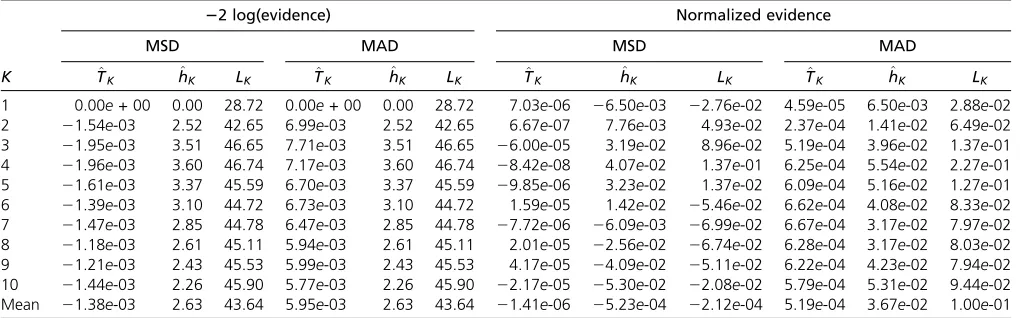
list of parameters). Each data set was then analyzed using the program MavericK1.0. This program is written in C++ and was designed specifically to carry out TI for structured pop-ulations via the algorithms described in the Appendix. In Table 1 Accuracy of estimation methods compared with the exact model evidence

22 log(evidence) Normalized evidence

MSD MAD MSD MAD

K T^K h^K LK T^K h^K LK ^TK ^hK LK T^K h^K LK

1 0.00e+ 00 0.00 28.72 0.00e+ 00 0.00 28.72 7.03e-06 26.50e-03 22.76e-02 4.59e-05 6.50e-03 2.88e-02 2 21.54e-03 2.52 42.65 6.99e-03 2.52 42.65 6.67e-07 7.76e-03 4.93e-02 2.37e-04 1.41e-02 6.49e-02 3 21.95e-03 3.51 46.65 7.71e-03 3.51 46.65 26.00e-05 3.19e-02 8.96e-02 5.19e-04 3.96e-02 1.37e-01 4 21.96e-03 3.60 46.74 7.17e-03 3.60 46.74 28.42e-08 4.07e-02 1.37e-01 6.25e-04 5.54e-02 2.27e-01 5 21.61e-03 3.37 45.59 6.70e-03 3.37 45.59 29.85e-06 3.23e-02 1.37e-02 6.09e-04 5.16e-02 1.27e-01 6 21.39e-03 3.10 44.72 6.73e-03 3.10 44.72 1.59e-05 1.42e-02 25.46e-02 6.62e-04 4.08e-02 8.33e-02 7 21.47e-03 2.85 44.78 6.47e-03 2.85 44.78 27.72e-06 26.09e-03 26.99e-02 6.67e-04 3.17e-02 7.97e-02 8 21.18e-03 2.61 45.11 5.94e-03 2.61 45.11 2.01e-05 22.56e-02 26.74e-02 6.28e-04 3.17e-02 8.03e-02 9 21.21e-03 2.43 45.53 5.99e-03 2.43 45.53 4.17e-05 24.09e-02 25.11e-02 6.22e-04 4.23e-02 7.94e-02 10 21.44e-03 2.26 45.90 5.77e-03 2.26 45.90 22.17e-05 25.30e-02 22.08e-02 5.79e-04 5.31e-02 9.44e-02 Mean 21.38e-03 2.63 43.64 5.95e-03 2.63 43.64 21.41e-06 25.23e-04 22.12e-04 5.19e-04 3.67e-02 1.00e-01

Shown are mean signed difference (MSD) and mean absolute difference (MAD) of various estimation methods compared with the exact value, obtained by brute force. Formulas forT^K;^hK;andLK are given in Equations 9, 4, and 5, respectively. Values are shown in log space (columns 2–7) and linear space after exponentiating and

normalizing to sum to 1 (columns 8–13). Values ofKhere denote the value used in the inference step, with each row being an average over 1000 simulations (a more detailed breakdown can be found inTable S1).

addition, MavericK1.0 implements certain features that lead to efficient and reliable exploration of the posterior, including solving the label switching problem via the method of Stephens (2000) (seeFile S2for further details of the main algorithm). The output of MavericK1.0 includes values of^hK;

LK;and the TI estimatorT^K:Calculation ofLKwas compared

extensively against Structure2.3.4 to ensure agreement. For the TI estimator the number of“rungs”used (the value ofr) was set to 50, while forh^KandLKthe analysis was repeated

50 times to obtain a global mean and standard error over replicates, thereby ensuring that the same computational ef-fort was expended for all methods. A total of 10,000 samples were obtained from the posterior distribution in each MCMC analysis, with a burn-in of 1000 iterations.

Figure 1 shows the results of one such analysis, in which the true number of demes wasK¼2:

It can be seen that both^hKandLKare negatively biased in

this example, leading to estimates of223logðevidenceÞthat are smaller than the true value. Any bias that is constant over

Kgoes away after transforming to a linear scale and normal-izing; however,^hKand particularlyLKstill give poor estimates

of the true posterior distribution.

The accuracy and precision of the different estimators was evaluated across all 1000 simulated data sets in the form of the mean signed difference (MSD) and the mean absolute differ-ence (MAD). The MSD measures the average differdiffer-ence be-tween the true and estimated values and hence can be considered a measure of bias, while the MAD measures the averageabsolutedifference and hence is influenced by both the bias and the precision of the estimator (small values rep-resent estimates that are both accurate and precise). Results are given in Table 1, broken down by the value ofKused in the inference step (a more detailed breakdown can be found inTable S1).

It can be seen that the average MAD of theLK estimator

after normalizing is0.1, while the MAD of theT^Kestimator

is 5:1931024 _{for the same computational effort. The} har-monic mean estimator is intermediate between these values, differing from the true evidence by0.04 on average. Based on these results we would expect estimates of the posterior distribution of K made using ^hK or LK to be qualitatively

different from the true posterior distribution.

Accuracy for larger data sets

Although the results in Table 1 are suggestive of a weakness in heuristic estimators, we are limited here to looking at small data sets in which the exact model evidence can be calculated by brute force. It is plausible based on these results that the bias in^hKandLKcould be amplified in small data sets due to a

lack of information and would cease to be a problem if more data were available. Here we therefore use larger simulated data sets to address the question of whether the TI method produces improvements that would be of practical impor-tance. Although we cannot calculate the true evidence by brute force here, the advantage of using simulated data sets is that we can generate observations from the exact model

used in the inference step and for aknownvalue ofK. We can then measure the proportion of times that the true value ofK

is correctly identified. As well as comparing the estimators

^

TK;^hK;andLK;in which the smallest value of the estimator

indicates the most likely model, we also compared Evanno’s

DK(Evannoet al.2005), in which the largest value indicates

the point of maximum curvature ofLK;and the AIC, BIC, and

DIC statistics, in which the smallest value indicates the

best-fitting model. Values of the DIC were calculated using the method of Spiegelhalteret al.(2002) (DIC S) as well as the method of Gelmanet al.(2004) (DIC G). To ensure that our results were not driven by a lack of information, larger data sets ofn¼200 diploid individuals atL¼10;20, and 50 loci were generated from the same without-admixture model used above. As before, 1000 simulated data sets were pro-duced withKranging from 1 to 10 (100 simulations each). MavericK1.0 was run under the without-admixture model Table 2 Percentage timesKcorrectly identified

K ^TK ^hK LK DK AIC BIC DIC S DIC G

10 loci

1 100.0 76.0 0.0 — 88.0 100.0 0.0 100.0

2 100.0 83.0 0.0 100.0 99.0 100.0 0.0 98.0

3 100.0 83.0 0.0 76.0 100.0 100.0 0.0 94.0

4 100.0 77.0 0.0 67.0 95.0 99.0 0.0 89.0

5 100.0 71.0 0.0 58.0 98.0 92.0 0.0 90.0

6 100.0 72.0 1.0 45.0 96.0 75.0 0.0 90.0

7 100.0 65.0 3.0 43.0 96.0 35.0 0.0 94.0

8 100.0 46.0 6.0 42.0 93.0 7.0 0.0 84.0

9 100.0 57.0 17.0 14.0 96.0 1.0 0.0 94.0

10 100.0 100.0 100.0 — 96.0 0.0 100.0 99.0

Mean 100.0 73.0 12.7 55.6 95.7 60.9 10.0 93.2 20 loci

1 100.0 100.0 0.0 — 95.0 100.0 0.0 89.0

2 100.0 100.0 2.0 100.0 100.0 100.0 0.0 86.0 3 100.0 100.0 64.0 95.0 100.0 100.0 10.0 92.0 4 100.0 99.0 85.0 93.0 100.0 100.0 44.0 97.0 5 100.0 98.0 90.0 97.0 100.0 100.0 70.0 100.0 6 100.0 92.0 88.0 94.0 100.0 100.0 78.0 100.0 7 100.0 94.0 85.0 93.0 100.0 94.0 84.0 99.0 8 100.0 91.0 87.0 97.0 100.0 73.0 78.0 100.0 9 100.0 87.0 82.0 88.0 100.0 26.0 70.0 97.0 10 100.0 100.0 100.0 — 100.0 3.0 100.0 100.0 Mean 100.0 96.1 68.3 94.6 99.5 79.6 53.4 96.0

50 loci

1 100.0 100.0 45.0 — 100.0 100.0 17.0 25.0

2 100.0 99.0 21.0 100.0 100.0 100.0 100.0 19.0 3 100.0 90.0 30.0 99.0 100.0 100.0 100.0 17.0 4 100.0 97.0 32.0 100.0 100.0 100.0 100.0 23.0 5 100.0 98.0 28.0 100.0 100.0 100.0 100.0 20.0 6 100.0 97.0 42.0 100.0 100.0 100.0 100.0 27.0 7 100.0 98.0 47.0 100.0 100.0 100.0 100.0 30.0 8 100.0 95.0 58.0 99.0 100.0 95.0 100.0 47.0 9 100.0 96.0 63.0 99.0 100.0 83.0 100.0 57.0 10 100.0 100.0 99.0 — 100.0 45.0 100.0 100.0 Mean 100.0 97.0 46.5 99.6 100.0 92.3 91.7 36.5

Shown is the percentage timesKis correctly identified by each method, broken down by the value ofKused when generating the data. Formulas forT^K;^hK;andLK

are given in Equations 9, 4, and 5, respectively, while formulas for AIC, BIC, DIC S;

and DICG are given inFile S1Equations 40, 43, 46, and 47, respectively. The

formula forDK can be found in Evannoet al.(2005).

with 1000 burn-in iterations and 10,000 sampling iterations. For the TI estimator 50 rungs were used, and forLK and^hK

the analysis was repeated 50 times.

Table 2 gives the proportion of times that the correct value ofKwas identified by each of the methods. It can be seen that the TI-based method of choosingKprovided 100% reliable results across all simulated data sets. Estimates ofKbased on

^

hK were less reliable, although still reasonable when the

number of loci was large, whereas estimates based on LK

were generally not reliable and particularly poor when the number of loci was small. This appears to be due to the well-documented tendency of LK to continually increase with

larger values ofK(Pritchardet al.2010), also giving the false impression that LK is highly accurate when K¼10 in this

example. Evanno’sDKmitigated this to some extent, but still

did not provide consistently reliable results (note that DK

cannot be calculated on the smallest or largest Kin any analysis as a consequence of how it is derived). Of the model comparison statistics the AIC was the most consis-tently reliable, providing accurate estimates across a range of simulations.

Returning to the question of whether the inaccuracy in^hK

andLKin Table 1 was driven by a lack of information, it can

be seen from Table 2 that the quantity of data certainly plays a role. However, the fact that TI provides reliable estimates across the range of simulations indicates that there is suffi -cient signal in the data to detect the value ofKeven in rela-tively small data sets. Thus, the increased precision of the TI approach is of practical as well as theoretical importance.

Reanalysis of white-footed mouse data

Our main reason for focusing on simulated data sets above is for the purposes of comparing different statistical methods under very controlled circumstances. By simulating data from the exact model used in the inference step we can tease apart the issue of whether inaccuracies are due to statistical prob-lems or simply a lack of modelfit to the data (the latter being ruled out). However, ultimately our interest lies in real-world analyses of population structure. Here the parameterKhas a less literal meaning and should be seen as a convenient way of summarizing the structure in the available data, rather than as an exact description of the number of demes.

To test MavericK1.0 in a realistic setting we reanalyzed data from a study by Munshi-South and Kharchenko (2010b), made available through the Dryad digital repository (Munshi-South and Kharchenko 2010a). The data consist of diploid genotypes at 18 putatively neutral microsatellite loci in 312 white-footed mice (Peromyscus leucopus), sampled from 15 distinct locations in and around New York City (see the original article for details). White-footed mice are known to be urban adaptors, and so the original study investigated the effects of urbanization and habitat fragmentation on the mouse population, concluding that there has been pervasive genetic differentiation and the emergence of strong popula-tion structure. The authors carried out a range of statistical tests, including but not limited to an analysis with Struc-ture2.3 under the admixture model with correlated allele frequencies and withainferred as part of the MCMC. They explored values ofKfrom 1 to 20 (repeating each analysis 10 times),finding that the meanLK peaked atK¼16 while

Evanno’sDK had peaks atK¼6 andK¼16;although

gen-erally the distribution of this statistic was complex (seefigure 2 in Munshi-South and Kharchenko 2010b).

We carried out a similar analysis in MavericK1.0, using TI to estimate the evidence for Kas well as using^hK andLK:We

used the same admixture model as in the original study, in whichais inferred as part of the MCMC; however, the correlated allele frequencies model is not implemented in MavericK1.0 and so we assumed a model of independent allele frequen-cies. For this reason our results are not directly comparable with those of the original study, although our assumptions are broadly similar. We exploredKfrom 1 to 20. When car-rying out TI we usedr¼21 rungs, and for the other estima-tion methods we took the mean and standard error over 21 replicates. For each MCMC analysis we ran 10 chains, each with 10,000 burn-in iterations and 50,000 sampling iter-ations, before trimming and merging chains to obtain 500,000 sampling iterations (we found that this gave better results than running one long chain).

The results of this analysis are shown in Figure 2. It can be seen thatLK increases smoothly withK, in a trend similar to

that found by Munshi-South and Kharchenko (2010b), the difference being that we find no peak at K¼16: The har-monic mean estimator increases rapidly until K¼5 but at Figure 2 Estimates of the model evidence for K¼1:20 obtained using (A) the Structure estimator LK;(B) the harmonic mean estima-tor^hK;and (C) the TI estimatorT^K: For A and B, solid points give the mean over 21 replicates and error bars give 95% confidence intervals calculated from the variance over replicates. For C the TI estimation procedure results in a single point estimate of the evidence and an estimate of the 95% confidence interval without the need to aver-age over replicates.

this point saturates and cannot distinguish between higher values of K. In contrast to both of these statistics, the TI estimator has a strong peak atK¼5 with narrow confidence intervals. Based on the arguments presented above we con-clude that this is the most accurate curve for the model evi-dence, and so K¼5 has the strongest support under this model. The posterior allocation plot for K¼5 is shown in Figure 3 (plots for all values of K can be found in Figure S1). Comparing this with figure 3 in Munshi-South and Kharchenko (2010b), we see some striking similarities—for example, the strong population differentiation in the Hunters Island and Willow Lake (a.k.a. Flushing Meadows) samples and the greater uncertainty in samples from the Black Rock Forest location. However, we also group together several populations that were previously found to be distinct, includ-ing locations 3, 4, 5, and 7 (all from the Bronx) and locations 8, 9, 11, and 15 (all from central Queens). The fact that we found evidence for fewer distinct populations than the orig-inal study may be due to our use of an uncorrelated allele frequencies model, although the geographical proximity of these regions gives us some confidence that this clustering is biologically plausible. Moreover, the striking difference be-tween Figure 2A and Figure 2C demonstrates that different estimation methods can lead to quantitatively different con-clusions even conditional on the same underlying model.

Discussion

Model-based clustering methods have proved extremely use-ful within population genetics. The probabilistic allocation of individuals to demes employed by programs such as Structure has made it possible to tease apart population subdivision within a wide range of organisms, including humans (Rosenberget al.2002; Liet al.2008; Tishkoffet al.2009), human pathogens (Falushet al.2003b), plants (Garriset al.

2005), and animals (Parkeret al.2004). However, these pos-terior assignments are always produced conditional on the known value of K. Choosing an appropriate value ofK is statistically much more challenging than estimating popula-tion assignments, as it involves a comparison between mod-els rather than simple parameter estimation within a given model. Thermodynamic integration offers a way to do this, providing estimates of the evidence forKthat are both accu-rate and precise. Our reanalysis of the white-footed mouse

data demonstrates that this is of practical as well as theoret-ical importance, with the potential to lead to quantitatively different conclusions about the data.

The main disadvantage of TI is the computational cost. Multiple MCMC chains are needed, each drawn from a dif-ferent version of the power posterior, to compute a single estimate of the model evidence. If the number of rungs is too low, then the trapezoidal rule step in (9) will not capture the shape of the underlying curve that it is approximating, leading to bias in the estimator. We must also be careful to take account of autocorrelation in the samples. This is dealt with automat-ically in MavericK1.0 through the use of effective sample size (ESS) calculations (see File S1for details), which result in estimates of the model evidence that are accurate even in the presence of autocorrelation. However, it is still the case that high levels of autocorrelation require us to obtain a large number of posterior draws, and so we cannot ignore autocor-relation completely. This is a particular problem for the ad-mixture model with afree to vary, where the much higher dimensionality of the model (compared with the without-admixture case) tends to result in poor MCMC mixing.

For this reason, TI may be suitable only for small- to medium-sized data sets of the sort analyzed here, at least for the time being. The use of TI for large SNP data sets—for example, data from the Human Genome Diversity Project (HGDP) analyzed by Liet al.(2008)—is therefore not prac-tically possible at this stage without devoting significant com-putational resources to the problem. Good results will tend to be obtained when applied to data sets on the order of hun-dreds of individuals and tens to hunhun-dreds of loci, depending on the parameter set used. Fortunately, the accuracy of some heuristic estimators and traditional model comparison statis-tics appears to improve for larger data sets, and so it may be possible to sidestep this issue. It is also worth noting that, when genetic markers are sufficiently dense, loci can no longer be considered independent, alternative approaches such as chromosome painting may be more appropriate (Lawsonet al.2012).

An important consequence of working with the model evidence is that we must be careful in our choice of priors. In ordinary parameter estimation it is common practice to use relatively uninformative priors—the logic being that the model should be free to be driven by the data and not by our prior assumptions. However, when calculating the evidence (as in Figure 3Posterior assignment of all 312 individuals into K¼5 clusters. Site names correspond to locations in and around New York City, and major landmasses are also given (the Black Rock Forest site is not within any of thefive New York City boroughs). Further details of sampling sites can be found in Munshi-South and Kharchenko (2010b).

Equation 3), the thinness of the prior has an effect that is not diminished by adding more data. This can result in models being unduly punished if the observed data are extremely un-likelya priori. For example, our use of independent Dirichlet priors on the allele frequencies in all populations can be con-sidered a fairly thin prior, as no combination of allele frequen-cies is any more likely than any othera priori. This will tend to result in conservative estimates ofK, as there is a large cost (in evidence terms) of adding more populations unless they can justify their existence by a commensurate increase in the like-lihood. Alternative model formulations, such as the correlated allele frequencies model of Falushet al.(2003a), may therefore be better at detecting subtle signals of population subdivision. This model is likely to feature in later versions of MavericK.

Finally, it is important to keep in mind that when thinking about population structure, we should not place too much emphasis on any single value ofK. The simple models used by programs such as Structure and MavericK are highly ideal-ized cartoons of real life, and so we cannot expect the results of model-based inference to be a perfect reflection of true population structure (see discussion in Waples and Gaggiotti 2006). Thus, while TI can help ensure that our results are statistically valid conditional on a particular evolutionary model, it can do nothing to ensure that the evolutionary model is appropriate for the data. Similarly—in spite of the results in Table 2—we do not advocate using the model ev-idence (estimated by TI or any other method) as a way of choosing the single“best”value ofK. The chief advantage of the evidence in this context is that it can be used to obtain the complete posterior distribution ofK, which is far more infor-mative than any single point estimate. For example, by aver-aging over the distribution of K, weighted by the evidence, we can obtain estimates of parameters of biological interest (such as the admixture parametera) without conditioning on a single population structure. Although one value ofKmay be most likelya posteriori, in general a range of values will be plausible, and we should entertain all of these possibilities when drawing conclusions.

The MavericK program and documentation can be down-loaded fromwww.bobverity.com/MavericK.

Acknowledgments

We are grateful to Jason Munshi-South and Katerina Kharchenko for making the data from their 2010 white-footed mouse analysis publicly available, to James Borrell for patiently testing early versions of the program, and to three anonymous reviewers whose suggestions substantially improved this article.

Literature Cited

Baele, G., P. Lemey, T. Bedford, A. Rambaut, M. A. Suchardet al., 2012 Improving the accuracy of demographic and molecular clock model comparison while accommodating phylogenetic un-certainty. Mol. Biol. Evol. 29: 2157_–2167.

Beerli, P., and M. Palczewski, 2010 Unified framework to evalu-ate panmixia and migration direction among multiple sampling locations. Genetics 185: 313–326.

Blanquart, S., and N. Lartillot, 2006 A Bayesian compound sto-chastic process for modeling nonstationary and nonhomoge-neous sequence evolution. Mol. Biol. Evol. 23: 2058–2071. Corander, J., P. Waldmann, and M. J. Sillanpää, 2003 Bayesian

analysis of genetic differentiation between populations. Genet-ics 163: 367–374.

Evanno, G., S. Regnaut, and J. Goudet, 2005 Detecting the num-ber of clusters of individuals using the software structure: a simulation study. Mol. Ecol. 14: 2611–2620.

Falush, D., M. Stephens, and J. K. Pritchard, 2003a Inference of population structure using multilocus genotype data: linked loci and correlated allele frequencies. Genetics 164: 1567_–1587. Falush, D., T. Wirth, B. Linz, J. K. Pritchard, M. Stephens et al.,

2003b Traces of human migrations in helicobacter pylori pop-ulations. Science_299:1582_–1585.

Falush, D., M. Stephens, and J. K. Pritchard, 2007 Inference of population structure using multilocus genotype data: dominant markers and null alleles. Mol. Ecol. Notes 7: 574_–578. Friel, N., and A. N. Pettitt, 2008 Marginal likelihood estimation

via power posteriors. J. R. Stat. Soc. Ser. B Stat. Methodol. 70: 589–607.

Garris, A. J., T. H. Tai, J. Coburn, S. Kresovich, and S. McCouch, 2005 Genetic structure and diversity inOryza satival. Genetics 169: 1631–1638.

Gelman, A., and X.-L. Meng, 1998 Simulating normalizing con-stants: from importance sampling to bridge sampling to path sampling. Stat. Sci. 13: 163–185.

Gelman, A., J. B. Carlin, H. S. Stern, and D. B. Rubin, 2004 Bayesian Data Analysis, 2nd edition. Chapman & Hall/CRC, Boca Raton, Florida.

Hubisz, M. J., D. Falush, M. Stephens, and J. K. Pritchard, 2009 Inferring weak population structure with the assistance of sample group information. Mol. Ecol. Resour. 9: 1322–1332. Huelsenbeck, J. P., and P. Andolfatto, 2007 Inference of popula-tion structure under a Dirichlet process model. Genetics 175: 1787–1802.

Huelsenbeck, J. P., P. Andolfatto, and E. T. Huelsenbeck, 2011 Structurama: Bayesian inference of population struc-ture. Evol. Bioinform. Online 7: 55.

Jombart, T., and C. Collins, 2015 A tutorial for discriminant analysis of principal components (dapc) using adegenet 2.0.0. Available at: http://adegenet.r-forge.r-project.org/

files/tutorial-dapc.pdf.

Kass, R. E., and A. E. Raftery, 1995 Bayes factors. J. Am. Stat. Assoc. 90: 773–795.

Lartillot, N., and H. Philippe, 2006 Computing Bayes factors using thermodynamic integration. Syst. Biol. 55: 195–207.

Lawson, D. J., G. Hellenthal, S. Myers, and D. Falush, 2012 Inference of population structure using dense haplotype data. PLoS Genet. 8: e1002453.

Lepage, T., D. Bryant, H. Philippe, and N. Lartillot, 2007 A general comparison of relaxed molecular clock models. Mol. Biol. Evol. 24: 2669–2680.

Li, J. Z., D. M. Absher, H. Tang, A. M. Southwick, A. M. Castoet al., 2008 Worldwide human relationships inferred from genome-wide patterns of variation. Science 319: 1100–1104.

Malécot, G., 1948 Mathématiques de l’Hérédité. Masson & Cie, Paris. Munshi-South, J., and K. Kharchenko, 2010a Data from: Rapid, pervasive genetic differentiation of urban white-footed mouse (peromyscus leucopus) populations in New York City. Dryad digital repository. Available at: http://dx.doi.org/10.5061/ dryad.1893.10.5061/dryad.1893

Munshi-South, J., and K. Kharchenko, 2010b Rapid, pervasive ge-netic differentiation of urban white-footed mouse (peromyscus

leucopus) populations in New York City. Mol. Ecol. 19: 4242– 4254.

Neal, R. M., 1994 Contribution to the discussion of“Approximate Bayesian inference with the weighted likelihood bootstrap”by Michael A. Newton and Adrian E. Raftery. J. R. Stat. Soc. B 56: 41–42.

Newton, M. A., and A. E. Raftery, 1994 Approximate Bayesian inference with the weighted likelihood bootstrap. J. R. Stat. Soc. B 56: 3–48.

Parker, H. G., L. V. Kim, N. B. Sutter, S. Carlson, T. D. Lorentzen et al., 2004 Genetic structure of the purebred domestic dog. Science_304:1160_–1164.

Pella, J., and M. Masuda, 2006 The Gibbs and split merge sampler for population mixture analysis from genetic data with incom-plete baselines. Can. J. Fish. Aquat. Sci. 63: 576–596.

Pritchard, J. K., M. Stephens, and P. Donnelly, 2000 Inference of population structure using multilocus genotype data. Genetics 155: 945–959.

Pritchard, J. K., X. Wen, and D. Falush, 2010 Documentation for structure software: version 2.3. Available at:http://pritchardlab. stanford.edu/structure_software/release_versions/v2.3.4/ structure_doc.pdf.

Raftery, A. E., M. A. Newton, J. M. Satagopan, and P. N. Krivitsky, 2006 Estimating the integrated likelihood via posterior simu-lation using the harmonic mean identity. Bayes. Stat.8:1–45.

Raj, A., M. Stephens, and J. K. Pritchard, 2014 Faststructure: variational inference of population structure in large SNP data sets. Genetics 197: 573–589.

Rannala, B., and J. L. Mountain, 1997 Detecting immigration by using multilocus genotypes. Proc. Natl. Acad. Sci. USA 94: 9197–9201.

Rosenberg, N. A., J. K. Pritchard, J. L. Weber, H. M. Cann, K. K. Kidd et al., 2002 Genetic structure of human populations. Science 298: 2381–2385.

Spiegelhalter, D. J., N. G. Best, B. P. Carlin, and A. Van Der Linde, 2002 Bayesian measures of model complexity and fit. J. R. Stat. Soc. Ser. B Stat. Methodol. 64: 583–639.

Stephens, M., 2000 Dealing with label switching in mixture mod-els. J. R. Stat. Soc. Ser. B Stat. Methodol. 62: 795–809. Tishkoff, S. A., F. A. Reed, F. R. Friedlaender, C. Ehret, A. Ranciaro

et al., 2009 The genetic structure and history of Africans and African Americans. Science 324: 1035_–1044.

Waples, R. S., and O. Gaggiotti, 2006 Invited review: What is a population? An empirical evaluation of some genetic methods for identifying the number of gene pools and their degree of connectivity. Mol. Ecol. 15: 1419_–1439.

Wright, S., 1949 The genetical structure of populations. Ann. Eu-gen. 15: 323_–354.

Communicating editor: N. A. Rosenberg

Appendix

MCMC Under the Without-Admixture Model

To carry out the TI estimation approach we need to be able to draw from the power posterior distribution. This is straightforward in the case of genetic mixtures and requires nothing more than a simple extension of existing MCMC algorithms. In the following we strive to bring our notation in line with previous studies wherever possible, but the complexities of certain likelihood functions also motivate us to define some new notation (see Table A1). It is worth noting, for example, that we will write individual genotypes in simple list form (as in Pritchardet al.2000), using the notationxilfor thelth locus of theith individual, but also in

allelic partition form (as in Huelsenbeck and Andolfatto 2007), using the notation sil:For example, a diploid individual

homozygous for the third allele at a particular locus can be writtenxil¼ ð3;3Þor equivalentlysil ¼ f0;0;2;0;0g;where there

arefive possible alleles to choose from in this example. Conditioning on the modelMKis also implicit throughout this section.

In the basic algorithm described by Pritchardet al.(2000) there are two free parameters to keep track of—the allocation of individuals to demes, denotedzhere, and the allele frequencies in allKdemes, denotedp:Under the assumptions of Hardy– Weinberg and linkage equilibrium it is possible to write the probability of the observed data given the known values of these free parameters, Prðxjz;pÞ:Combining this likelihood with a Dirichletðll1;. . .;llJlÞprior on the allele frequencies at each locus,

we can derive the conditional posterior distribution of the allele frequencies given the known group allocation, Prðpjx;zÞ: Alternatively, multiplying by an equal 1=K prior on the allocation of individuals to demes, we can derive the conditional posterior distribution of the group allocation given the known allele frequencies, Prðzjx;pÞ:Algorithm 1 of Pritchardet al.

(2000) works by alternately sampling from each of these conditional distributions, resulting (after sufficient burn-in) in a series of draws from the full posterior distribution. More often than not we are interested in the posterior allocation, in which case the posterior allele frequencies can simply be ignored.

However, as stated in the original derivation of Rannala and Mountain (1997) and reiterated by later authors (Corander

et al.2003; Pella and Masuda 2006; Huelsenbeck and Andolfatto 2007), it is possible to integrate over the allele frequencies analytically, thereby greatly reducing the dimensionality of the problem. The new likelihood, conditional only on the group allocation, can be written

PrðxjzÞ ¼Y K

k¼1

YL

l¼1

Gðll0Þ

Gðll0þykl0Þ

YJl

j¼1

GðlljþykljÞ

GðlljÞ  

(A1)

(see Table A1 for parameter definitions). This expression is extremely useful to us, as it means the likelihood can be calculated without having to take into account an explicit representation of the unknown allele frequencies—our uncertainty in the allele frequencies has already been integrated out of the problem.

Rather than using (A1) directly, later authors including Coranderet al.(2003), Pella and Masuda (2006), and Huelsenbeck and Andolfatto (2007) used this analytical solution to define an efficient MCMC algorithm. Dividing the probability of the data x by the probability of the data with theith observation removed, denotedxð2iÞ_{;we obtain the conditional probability of}

observationigiven all others. Using the fact thatykl¼y

ð2iÞ

kl þsil;we obtain

Prxijzi¼k;yð2 iÞ

k

¼YL

l¼1

Gll0þyð_kl2₀iÞ

Gll0þy_klð2₀iÞþsil0

YJl

j¼1

Glljþy_kljð2iÞþsilj

Glljþy_kljð2iÞ

: (A2)

Computing (A2) for allkand normalizing, we obtain the conditional posterior probability that individualibelongs to demek:

Pr

zi¼kjxi;yð_k2iÞ

¼ ð1=KÞPr

xijzi¼k;yð2 iÞ

k

XK

u¼1ð1=KÞPr

xijzi¼u;yðu2iÞ

: (A3)

By repeatedly drawing new group allocations for all individuals from (A3), we obtain a series of draws from the posterior distribution without ever needing to invoke the unknown allele frequencies. Thus, the two-step algorithm of Pritchardet al.

(2000) can be reduced to the more efficient one-step algorithm of Coranderet al.(2003).

The reason these results are pertinent to our problem is that we can make use of the same gains in efficiency when designing an MCMC algorithm for the purposes of TI. In fact, the only difference when carrying out TI is that the likelihood in (A1) should be raised to the powerb, allowing us to draw from the power posterior. On making this change wefind that the conditional

posterior distribution in (A2) should also be raised to the powerb[this follows from the fact that (A2) can be derived as a ratio of two ordinary likelihoods]. Thus, we arrive at a new expression for the probability of individualibeing assigned to groupk:

P_b

zi¼kjxi;yð_k2iÞ

¼ ð1=KÞPr

xijzi¼k;yðk2iÞ

_b

XK

u¼1ð1=KÞPr

xijzi¼u;yðu2iÞ

_b: (A4)

By repeatedly sampling new group allocations for all individuals from (A4), we obtain a series of allocation vectors drawn from the power posterior (note that whenb¼0;we are essentially drawing from the prior). The likelihood of each vector can then be computed using (A1), at which point we have everything we need to calculateD^b as in (8). Carrying out this entire

procedure for a range of valuesbi;we obtain a series of pointsD^bi that can be used to calculate the TI estimator^TK;as in

(9). The complete TI algorithm for the model without admixture can be defined as follows: Algorithm 1 (without admixture)

1. Forrdistinct values ofbispanning the interval½0;1

a. Perform MCMC by repeatedly drawing from (A4) for alli2 f1;. . .;ng:This results (after discarding burn-in) intdraws from the power posterior group allocation.

b. Calculate the likelihood of each group allocation, using (A1).

c. CalculateD^bias the average log-likelihood, as in (8). If calculating the variance of the estimator, calculateV^biusing the

formula inFile S1, taking care to use an appropriate value of the ESS.

2. Use the valuesD^bi to calculateT^Kin a suitable numerical integration scheme, for example using the trapezoidal rule as

in (9).

MCMC Under the Admixture Model

The model with admixture described by Pritchardet al.(2000) is slightly complicated by the fact that each gene copy is free to originate from a different deme. However, we can still apply the same basic logic described above to arrive at a simple one-step algorithm for sampling from the power posterior. First, we note that the probability of the data conditional on the known group allocation is identical in this model to the probability in the without-admixture model and is given by (A1). This is true because we make the same assumption that gene copies are drawn independently from demes, and we apply the same Dirichlet priors on allele frequencies, meaning thefinal likelihood does not change. The difference in the admixture model is that the group allocation takes place at the level of the gene copy, rather than at the level of the individual, and so the valueszilaare no longer

restricted to being the same for allðl;aÞ:This is reflected in theykvalues used to keep track of the gene copies allocated to a

particular deme, which are now free to contain only a partial contribution of the genome of each individual.

Following the same approach as for the without-admixture model, we can obtain the conditional probability of gene copyxila

by dividing through the probability of the complete data by the probability of the data with this element removed [denoted xð2ilaÞ_{]. Most of the terms in the resulting expression cancel out, leading to the following simple result:}

Pr

xilajzila¼k;yð2 ilaÞ

k

¼ llxilaþy ð2ilaÞ

klxila ll0þyð2

ilaÞ

kl0

0 @

1

A_: (A5)

As before, this likelihood should be combined with the prior probability of assignment to each deme. If the admixture proportions for individualiare given by the vectorqi;then, under the assumptions of the model described by Pritchardet al.(2000), the

number of gene copies in this individual that are allocated to each deme can be considered a multinomial draw from qi:

Integrating over a Dirichletða;. . .;aÞprior on these frequencies, we obtain

Prðzjv;aÞ ¼Y n

i¼1

GðKaÞ

GðKaþvi0Þ

YK

k¼1

GðaþvikÞ

GðaÞ : (A6)

We can use this expression to write down the prior probability of gene copyaat locuslin individualibeing allocated to demek, conditional on the allocations of all other gene copies:

Pr

zila¼k   vði2ilaÞ;a

¼ aþv

ð2ilaÞ

ik Kaþvð_i02ilaÞ

!

: (A7)

Bringing together the prior with the likelihood raised to the powerb, we obtain the following expression for the power posterior probability of an individual gene copy being allocated to demek:

P_bzila¼kjxila;yð2 ilaÞ

k ;v

ð2ilaÞ

i ;a

¼ Pr

zila¼kjvði2ilaÞ;a

Pr

xilajzila¼k;yðk2ilaÞ

_b

XK

u¼1Pr

zila¼ujvði2ilaÞ;a

Pr

xilajzila¼u;yðu2ilaÞ

_b: (A8)

By repeatedly sampling new allocations for all gene copies at all loci within all individuals (i.e., allzila), we obtain a series of

draws from the power posterior group allocation under the admixture model. Again, this algorithm is made more efficient by the fact that the unknown allele frequencies in all populationsandthe unknown admixture proportions in all individuals have been integrated out of the problem at an early stage.

A common extension to the basic admixture model is to leaveaas a free parameter, updating it as part of the MCMC. This can be accommodated within the TI framework by using a simple Metropolis–Hastings step. Ifa9is a new value ofa, drawn from some suitable proposal distributiongða9 aÞ;then the acceptance probability under Metropolis–Hastings is given by

Pr

a/a9¼min 1;Pr

zjv;a9gaja9

Prðzjv;aÞgða9jaÞ !

: (A9)

Note that the core probability that drives this expression is thepriorprobability of the allocationz;which is given in (A6). The actual probability of the data—i.e., the expression that is raised to the powerbin the power posterior calculation—does not feature here. Thus, we can use the same Metropolis–Hastings step to updateairrespective of the value ofb.

The complete TI algorithm for the model with admixture can be defined as follows: Algorithm 2 (with admixture)

1. Forrdistinct values ofbispanning the interval½0;1

a. Perform MCMC by repeatedly drawing from (A8) for all gene copies at all loci in all individuals (alla;l;i). Ifais a free parameter, then update this value using a Metropolis–Hastings step, as in (A9). This results (after discarding burn-in) int

draws from the power posterior group allocation.

b. Calculate the likelihood of each group allocation, using (A1).

c. CalculateD^bias the average log-likelihood, as in (8). If calculating the variance of the estimator, calculateV^biusing the

formula inFile S1, taking care to use an appropriate value of the ESS.

2. Use all the valuesD^bito calculate^TKin a suitable numerical integration scheme, for example using the trapezoidal rule as in

(9).

Finally, we note that the expressions derived in this section can be used to obtain the exact model evidence by brute force in restricted settings. For example, focusing on the model without admixture, we could sum over the likelihood of all possible group allocations to obtain the true model evidence,

PrðxÞ ¼X z  

PrðxjzÞPrðzÞ; (A10)

where PrðxjzÞis given by (A1), and for this model PrðzÞ ¼1=Kn_{for all group allocations. Although this is possible in theory, the}

sheer number of allocations that are required to sum over makes this method impractical in all but the simplest situations. Even if we exploit redundancies in the labeling of different allocations, we are still restricted to values ofnandKnot much.10. This method is therefore only really useful as a way of checking the accuracy of other estimation methods.

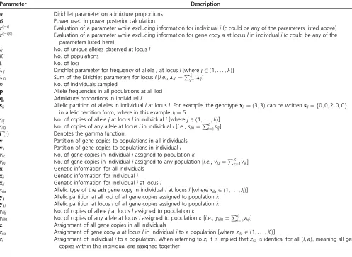
Table A1 Definitions of parameters used in this study

Parameter Description

a Dirichlet parameter on admixture proportions b Power used in power posterior calculation

cð2iÞ _{Evaluation of a parameter while excluding information for individuali(ccould be any of the parameters listed above)} cð2ilpÞ _{Evaluation of a parameter while excluding information for gene copyaat locuslin individuali(ccould be any of the}

parameters listed here)

Jl No. of unique alleles observed at locusl

K No. of populations

L No. of loci

llj Dirichlet parameter for frequency of allelejat locusl[wherej2 ð1;. . .;JlÞ]

ll0 Sum of the Dirichlet parameters for locusl[i.e.,ll0¼PJ_jl¼1llj]

n No. of individuals sampled

p Allele frequencies in all populations at all loci qi Admixture proportions in individuali

sil Allelic partition of alleles in individualiat locusl. For example, the genotypexil¼ ð3;3Þcan be writtensil¼ f0;0;2;0;0g

in allelic partition form, where in this exampleJl¼5

silj No. of copies of allelejat locuslin individuali[wherej2 ð1;. . .;JlÞ]

sil0 No. of copies of any allele at locuslin individuali[i.e.,sil0¼PJ_jl¼1silj]

GðÞ Denotes the gamma function.

v Partition of gene copies to populations in all individuals vi Partition of gene copies to populations in individuali vik No. of gene copies in individualiassigned to populationk

vi0 No. of gene copies in individualiassigned to any population [i.e.,vi0¼PK_k¼1vik] x Genetic information for all individuals

xi Genetic information for individuali

xil Genetic information for individualiat locusl

xila Allelic type of theathgene copy in individualiat locusl[wherexila2 ð1;. . .;JlÞ] yk Allelic partition at all loci of all gene copies assigned to populationk

ykl Allelic partition at locuslof all gene copies assigned to populationk yklj No. of copies of allelejat locuslassigned to populationk

ykl0 No. of copies of any allele at locuslassigned to populationk[i.e.,ykl0¼PJ_j¼l1yklj] z Assignment of all gene copies in all individuals

zila Assignment of gene copyaat locuslin individualito a population [wherezila2 ð1;. . .;KÞ]

zi Assignment of individualito a population. When referring toziit is implied thatzilais identical for allðl;aÞ;meaning all gene copies within this individual are assigned together

GENETICS

Supporting Information

www.genetics.org/lookup/suppl/doi:10.1534/genetics.115.180992/-/DC1

Estimating the Number of Subpopulations (

K

) in

Structured Populations

Robert Verity and Richard A. Nichols

Table S1. Mean signed difference and mean absolute difference for all values of K explored in the first simulated data analysis. (.xlsx, 59 KB)

Available for download as a .xlsx file at:

File S

1:

Derivation

of

Evidence

Estimators

and

Model

Comparison

Statistics

Supplementary

material

for

the

paper

Estimating

K

in

Genetic

Mixture

Models

Robert

Verity,

Richard

A.

Nichols

Contents

1 Problem Specification 2

2 Direct Estimators of the Model Evidence 2

2.1 The Harmonic Mean Estimator . . . 2 2.2 Thermodynamic Integration . . . 3

3 Approximations to the Model Evidence 5

3.1 The ‘Structure estimator’ LK . . . 5

3.2 The BIC . . . 6

4 General Model Comparison Statistics 10

4.1 The AIC . . . 10 4.2 The BIC (again) . . . 11 4.3 The DIC . . . 11

1

Problem Specification

The purpose of this supplementary text is to gather together in one place the mathematical derivation of the various estimators and model comparison statistics that are implemented in the main text. We present the rationale for each method in a manner that emphasises the common underpinnings that connect the different approaches.

From a notational point of view let us assume a data vector x, a model M, and a parameter vector θ of length d(i.e. there are d free parameters under the model). The likelihood under the model can be written Pr(x|θ,M), and the prior can be written Pr(θ| M). The model evidence can be obtained from the likelihood and the prior as follows:

Pr(x| M) =

Z

θ

Pr(x|θ,M)Pr(θ| M)dθ . (1)

Some of the model comparison statistics described below can be considered direct estimators of, or approximations to, this quantity. Others are derived from entirely different perspectives.

2

Direct Estimators of the Model Evidence

2.1

The Harmonic Mean Estimator

The harmonic mean estimator can be derived from Bayes’ rule, which when written in reverse reads

Pr(x|θ,M)Pr(θ| M)

Pr(x| M) = Pr(θ|x,M). (2)

Dividing both sides of (2) by the likelihood Pr(x|θ,M) and integrating over

θ we obtain

1

Pr(x| M) =

Z

θ

Pr(θ|x,M)

Pr(x|θ,M) dθ . (3)

Replacing the integral on the RHS of (3) by its Monte Carlo estimator we obtain

1

Pr(x| M) ≈ 1

t t X

m=1

1 Pr(x|θm,M)

, (4)

where θm for m ∈ {1, . . . , t} represents a series of draws from the posterior

distribution of θ. Taking the reciprocal of (4) we arrive at the harmonic

mean estimator, ˆh:

ˆ

h = ₁ 1

t Pt

m=1

1

Pr(x|θm,M)

, (5)

as defined by Newton and Raftery (1994). Although elegant in its simplicity, and technically unbiased, this estimator is highly unstable, often having in-finite variance. See Raftery et al. (2006) for constructive suggestions on how to avoid some of the problems inherent in this estimator.

2.2

Thermodynamic Integration

Thermodynamic Integration (TI) provides direct estimates of the model ev-idence that are unbiased and have finite and quantifiable variance. The method exploits the ‘power posterior’ (Friel and Pettitt, 2008), defined as follows:

Pβ(θ|x,M) =

Pr(x|θ,M)β Pr(θ| M)

u(x|β,M) . (6)

where u(x|β) is the following normalising constant:

u(x|β,M) =

Z

θ

Pr(x|θ,M)βPr(θ| M)dθ, (7)

(in subsequent expressions the conditioning on the model M will be su-pressed). The crucial step in the TI method is the following derivation:

d

dβlog[u(x|β)] =

1

u(x|β)

d

dβu(x|β),

= 1

u(x|β)

Z

θ d

dβPr(x|θ)

β_{Pr(θ)dθ ,}

= 1

u(x|β)

Z

θ

Pr(x|θ)βlog[Pr(x|θ)] Pr(θ)dθ,

=

Z

θ

log[Pr(x|θ)]Pr(x|θ)

β_Pr(θ)

u(x|β) dθ ,

=

Z

θ

log[Pr(x|θ)]Pβ(θ|x)dθ,

= Eθ|x,β

h

log[Pr(x|θ)]

i

. (8)

In other words, the gradient of log[u(x|β)] is equivalent to the expected log-likelihood of the parameterθ, where the expectation is taken over the power posterior. It is easy to demonstrate that the integral of (8) with respect to

β over the range [0,1] is equal to the logarithm of the model evidence:

Z 1

0 d

dβlog[u(x|β)]dβ = log[u(x|β= 1)]−log[u(x|β= 0)],

= log[Pr(x)], (9)

where we have made use of the fact that u(x|β= 1) is equal to the model evidence, and u(x|β= 0) is equal to the integral over the prior, which is 1 by definition. Therefore if we could calculate the expectation in (8) and if we could integrate this expectation over β ∈ [0,1] then we would arrive at the logarithm of the model evidence.

Thermodynamic integration is essentially a numerical approximation to this scheme. Let θβ_m for m ∈ {1, . . . , t} represent a series of independent draws from the power posterior with power β. Then the expectation in (8) can be estimated using the Monte Carlo estimator Dbβ, defined as follows:

b

Dβ =

1

t t X

m=1

log

h

Pr(x|θβ_m)

i

. (10)

Turning to the integral in (9), we cannot carry out this integration step analytically, but we can approximate it using the values Dbβ in a simple

numerical integration technique, such as the trapezoidal rule. For example, if the valuesβi = (i−1)/(r−1) fori={1, . . . , r}represent a series of equally

spaced powers spanning the interval [0,1], where r denotes the number of ‘rungs’ used (r≥2), then the integral in (9) can be approximated using

b

T =

r−1

X

i=1

1

2(Db_βi+1+Db_βi)

r−1 ,

= _r−11 1₂Db_β1 +1₂Db_βr+

r−1

X

i=2

b Dβi

. (11)

There are two sources of error in this estimator. First, there is ordinary statistical error associated with replacing (8) by its Monte Carlo estimator, and second, there is discretisation error caused by replacing a continuous integral with a numerical approximation. Both of these sources of error are quantified in Lartillot and Philippe (2006). In the example above the sampling variance of the estimator can be calculated using

Var[Tb] = _(r−1)1 2

1

4Var[Db_β1] + 1₄Var[Db_βr] +

r−1

X

i=2

Var[Db_βi]

, (12)

where the sampling variance of individual elements is obtained by dividing the variance by the MCMC effective sample size (ESS):

Var[Db_β]≈ b Vβ

ESS , (13)

b

Vβ = _t−11

t X

m=1

loghPr(x|θβ_m)i−Db_β

2

. (14)

The ESS is a crucial quantity in this expression. MCMC draws are often highly auto-correlated, meaning the effective number of independent samples is often much smaller than the number of samples. In order to obtain reliable estimates of the variance inTbwe must take this autocorrelation into account. A standard method is to calculate the ESS directly from the autocorrelation of the MCMC chain:

ESS = t 1 + 2P∞

l=1ρl

, (15)

whereρlgives the autocorrelation in the log-likelihood atllags. This method

is implemented within MavericK1.0, meaning autocorrelation is

automat-ically taken into account in estimates of the model evidence.

The sampling variance ofDbβ – and therefore the sampling variance of the

final estimator Tb – can be reduced be increasing the number of effectively independent draws from the posterior. This involves either increasing the raw number of draws, or improving the mixing of the MCMC to achieve greater independence. The discretisation error can also be kept within bounds. As noted by Friel et al. (2013), the curve traced by Eθ|x,β

h

log[Pr(x|θ)]i is always-increasing withβ, meaning there are strict upper and lower bounds on the error that is possible given a series of known values distributed along this curve (and ignoring interactions between statistical error and discretisation error). These bounds can be quantified, leading to an estimate of the worst-case scenario discretisation error. In practice we find that these estimates are too pessimistic to be useful, and prefer to simply examine the shape of the estimated curve to ensure that sufficient rungs have been used to capture the curvature.

3

Approximations to the Model Evidence

3.1

The ‘Structure estimator’

LK

The heuristic estimator LK (our notation), described by Pritchard et al.

(2000) and implemented in the program _Structure, is closely connected to

the harmonic mean estimator, but designed to avoid some of the problems inherent in the original method. As with many model comparison statistics, it can be derived from the Bayesian deviance, defined as -2 times the log-likelihood:

D(θ) = −2 log [Pr(x|θ,MK)] . (16)

(The notationMK has been used here to emphasise the connection with the

value of K, although in general this method can be applied to any model). The Bayesian deviance is a function of θ, and can therefore be calculated for any chosen value of θ – for example, it could be calculated from the poste-rior draws θm described earlier. The derivation of LK revolves around the

assumption that the values D(θm) are approximately normally distributed.

Note that this is not the same as assuming that the log-likelihood is normally distributed – rather, it assumes that the log-likelihood of a series of posterior draws is approximately normally distributed. The mean and variance of this normal distribution can be estimated in the usual way:

ED(θ)|x ≈ 1 t

t X

m=1

D(θm) = ˆµ , (17)

VarD(θ)|x ≈ 1

t−1

t X

m=1

(D(θm)−µˆ)2 = ˆσ2 . (18)

If the valuesD(θm) are indeed drawn from a Normal(ˆµ,σˆ2) distribution then

it follows from a simple transformation of (16) that the values 1/Pr(x|θm,MK)

must be drawn from a Lognormal(ˆµ/2,σˆ2/4) distribution. The expectation of this distribution is given by expnµ₂ˆ +σˆ₈2o, and the RHS of equation (4) can be seen an estimator of this expected value. It follows that

1

Pr(x| M_K) ≈ exp

ˆ

µ

2 + ˆ

σ2

8

, (19)

from which we obtain the heuristic estimator LK:

−2 log [Pr(x| MK)] ≈ µˆ+

ˆ

σ2

4 = LK . (20)

3.2

The BIC

The Bayesian Information Criterion (BIC) can be understood as a heuristic estimator of the model evidence, or as a general model choice criterion. In this section we deal with the former interpretation.

The derivation of the BIC as an estimator of the model evidence relies on several assumptions, and hence definitions of the BIC tend to vary slightly from text to text depending on which assumptions are used. The version presented here attempts to bridge the gap between these different definitions, and is based on the excellent explanation by Raftery (1995).

First, let us define the function g(θ) as the logarithm of the prior times the likelihood:

g(θ) = log [Pr(x|θ,M)Pr(θ| M)] . (21)

Note that the true model evidence is equal to the integral of exp{g(θ)} over θ. The first step in the BIC derivation is to assume that g(θ) is well-approximated by a second order Taylor series expansion about the maximum value ˜θ

g(θ) ≈ g(˜θ) + (θ−θ˜)T_g0_{(˜θ) +}1

2(θ−˜θ)Tg

00_{(˜θ)(θ−θ˜), (22)}

where g0(θ) and g00(θ) represent the first and second derivatives of the orig-inal function. The g0(θ) term in (22) must equal zero (the gradient at the maximum value ˜θ is zero by definition). Exponentiating the remaining terms we find that

Pr(x|θ,M)Pr(θ| M) ≈ expg(˜θ) exp−1

2(θ−θ˜)

T_{H(θ−θ˜) , (23)}

where ˜H =−g00(˜θ) is the hessian matrix for the function g(θ), evaluated at the point ˜θ. The quantity on the RHS of (23) is proportional to the multi-variate normal density. Hence, we can say that the first assumption of the BIC is that the posterior distribution is approximately normally distributed about the maximum. Integrating (23) over θ we obtain

Pr(x| M) ≈ exp g(˜θ)

Z

θ

exp−1

2(θ−θ˜)TH˜(θ−˜θ) dθ ,

= exp

g(˜θ) (2π)d2H˜

−1

2 _{, (24)}

where |H˜| indicates the determinant of the matrix ˜H (recall that d denotes the number of free parameters in the model, hence we have a d×d Hessian matrix). Taking logarithms and making use of (21) we obtain

logPr(x| M) ≈ logPr(x|θ˜,M)+ logPr(˜θ| M)+ d₂log[2π]

−1

2log

H˜

. (25)

Next, we assume that the maximum a posteriori value ˜θ is approximately equal to the maximum likelihood value ˆθ. Similarly, we assume that the