Structural Optimization of Cold-Formed Steel Frames to AISI-LRFD

Structural Optimization of Cold-Formed Steel

Frames to AISI-LRFD

Serdar Carbas1

Assistant Professor, Department of Civil Engineering, Karamanoglu Mehmetbey University, Karaman, Turkey1

ABSTRACT: The construction industry, from harvesting raw materials, transport, manufacturing, to the actual construction of buildings, has a significant and negative impact on the environment. The construction of buildings not only produces more waste, but also requires more transport and electricity (emissions), and often results in landscape damage, ecological disruption, habitat destruction, and/or deforestation. Utilizing cold-formed steel frame systems in construction supplies sustainability since this kind of framing are made out of thin-walled sections. Nowadays, there are a variety of metaheuristics developed for minimum weight design of cold-formed steel frames.In this study, the biogeography-based optimization (BBO) algorithm is used to select the cold-formed thin-walled C-sections listed in AISI-LRFD (American Iron and Steel Institution-Load and Resistance Factor Design) in such a way that the design constraints specified by the code are satisfied and the weight of the cold-formed steel frame is the minimum. It is shown that BBO algorithm out performs other metaheuristic technique in the design example considered.

KEYWORDS: Structural optimization, Cold-formed steel frames, Biogeography-based optimization, AISI-LRFD.

I. INTRODUCTION

Buildings are responsible for almost half of the world’s carbon emissions, half of its water consumption, around a third of its landfill waste and a quarter of all raw materials used in the economy (www.isover.com 2016). This means that the world’s sustainable development targets cannot be met without a fundamental change to the way in which buildings are designed, constructed and operated. The targets for greenhouse gas emission reductions and the drive for buildings present a huge challenge to the construction industry. The usage of steel in buildings is the best economical solution among different types of construction materials to overcome this challenge (www.greenmaltese.com 2016).

Especially, with the rapid development in industrial sector in the world, there is a high demand for clear span buildings to cater for the factories with advance technology production lines as well as for the warehouses. Cold-formed steel framing is the best solution for large clear spans and is the most popular structural form used in the construction industry, recently. It offers an economical solution to medium to large spans and the most important feature is the saving on material and construction time which is a main concerns of most the clients. However, to get the optimum solution in cold-formed steel frames there are several key factors, namely design limitations, to consider during the design stage (Yu and La Boube 2010).

Almost all design problems in engineering can be considered as optimization problems and thus require optimization techniques to solve. However, as most real-world problems are highly nonlinear, traditional optimization methods usually do not work well. The current trend is to use metaheuristic optimization methods to overcome such nonlinear optimization problems. Metaheuristic algorithms have gained great popularity in recent years (Saka et al. 2016). The popularity of nature-inspired metaheuristic algorithms can be attributed to their good characteristics because these algorithms are simple, flexible, efficient, and adaptable, and yet easy to implement. Such advantages make them versatile to tackle with a wide range of optimization problems without much preliminary information about the problem to be solved. Metaheuristic algorithms play significant role in the optimum design of complex engineering problems when analytical approaches and traditional methods are not effective for solving nonlinear design problems in different fields of civil engineering (Hasançebi et al. 2009, 2010).

popularity since the algorithm reveals itself due to its capacity of obtaining a near-global optimum especially in problems with large amount of design variables. This technique has been featly implemented a broad array of engineering and mathematical optimization problems (Boussaid et al. 2012, Rajasomashekar and Aravindhababu 2012, Kima et al. 2012, Saka et al. 2015).In this study, the BBO based design algorithm selects the cold-formed thin-walled C-sections listed in AISI-LRFD (American Iron and Steel Institution 2002, Load and Resistance Factor Design 1991)in such a way that the design constraints that are the displacement limitations, inter-story drift restrictions, effective slendernessratio, strength requirements for beams and combined axial and bending strengthrequirements including the elastic torsional lateral buckling for beam-columns, specified by the code are satisfied and the weight of the cold-formed steel frame is the minimum. The effectiveness of the proposed design algorithm is demonstrated on a design example.

II. DESIGNOPTIMIZATIONOFCOLD-FORMEDSTEELFRAMESTOAISI-LRFD

The selection of cold-formed thin-walled C-sections for the members of steel frame is required to be carried out in such a way that the frame with the selected C-sections satisfies the serviceability and strength requirements specified by the code of practice while the economy is observed in the overall or material cost of the frame. When the constraints are implemented from AISI-LRFD in the formulation of the design problem the following discrete programming problem is obtained.

Find a vector of integer values

I

(Eqn. 1) representing the sequence numbers of C-sections assigned to ng member groups

to minimize the weight (

W

) of the frame

Subject to

 Serviceability Constraints:

where, δjlis the maximum deflection of jth member under the lth load case, L is the length of member, nsm is the total number of members where deflections limitations are to be imposed, nlc is the number of load cases,His the height of the frame, njtop is the number of joints on the top story, Δtopjl is the top story displacement of the jth joint under lth load

T

I _{= I , I , ..., Ing}



_

_{1 2}



_

(1)

MinimizeW = ng m_knkL_i

k=1 i=1 (2)

1.0 0 ,    /

1, 2, , ,   1, 2, , jl

L Ratio

j nsm l nlc



 

   

(3)

1.0 0 ,    /

1, 2, , ,   1, 2, , top

jl

H Ratio

j nj_top l nlc

 

   



(4)

1.0 0 ,    /

1, 2, , ,   1, 2, , oh

jl

h Ratio

sx

j n_st l nlc



 

   

case, nstis the number of story, nlc is the number of load cases and Δohjlis the story drift of the jth story under lth load case, hsx is the story height and Ratiois limitation ratio for lateral displacements described inASCE Ad Hoc Committee report (Ad Hoc Committee on Serviceability 1986). According to this report, the accepted range of drift limits by first-order analysis is 1/750 to 1/250 times the building height H with a recommended value of H/400. The typical limits on the inter-story drift are 1/500 to 1/200 times the story height. 1/400 is used in this study.

 Strength Constraints:Combined Tensile Axial Load and Bending

It is stated in AISI-LRFD that when a cold-formed members are subject to concurrent bending and tensile axial load, the member shall satisfy the interaction equations given C5.1 of AISI which is repeated in Eqns. 6 and 7,

where;

Tu= required tensile axial strength [factored tension].

Øt= 0.95 (LRFD).

Tn= nominal tensile axial strength [resistance].

Mux,Muy= the required flexural strengths [factored moments] with respect to centroidal axes.

Øb = for flexural strength [moment resistance] equals 0.90 or 0.95 (LRFD).

Mnxt,Mnyt = SftFy (where, Sftis the section modulus of full unreduced section relative to extreme tension fiber about

appropriate axis and Fyis the design yield stress).

Mnx,Mny= nominal flexural strengths [moment resistances] about centroidal axes.

 Strength Constraints: Combined Compressive Axial Load and Bending

It is stated in AISI-LRFD that when a cold-formed members are subject to concurrent bending and compressive axial load, the member shall satisfy the interaction equations given in C5.2 of AISI which is repeated in Eqns. 8 to 10.

For Pu 0.15

P c n

  ,

For Pu 0.15

P c n

  ,

1.0 M

P_u M_ux uy

P M M

c n _b nx _b ny

    (10)

where,

Pu= required compressive axial strength [factored compressive force].

Øc= 0.85 (LRFD).

Mux,Muy= the required flexural strengths [factored moments] with respect to centroidal axes of effective section.

Øb = for flexural strength [moment resistance] equals 0.90 or 0.95 (LRFD).

Mnx,Mny = the nominal flexural strengths [moment resistances]about centroidal axes and 1.0

M

M_ux uy T_u

M_nxt M_{nyt tTn}

b b

    (6)

1.0

M

M_ux uy T_u

M_nx M_{ny t}T_n

b b

    (7)

1.0

C M

P_u C_mxM_ux my uy

P M M

c n _b nx x _b ny y

      (8)

1.0 M

P_u M_ux uy

P M M

c no b nx b ny

where,

2

2

( )

EI x P

Ex _{K L}

x x



 ,

2

2

( )

EI y PE_y

K L_{y y}



 (12)

where,

Ix= moment of inertia of full unreduced cross section about x axis.

Kx= effective length factor for buckling about x axis.

Lx= unbraced length for bending about x axis.

Iy= moment of inertia of full unreduced cross section about y axis.

Ky= effective length factor for buckling about y axis.

Ly= unbraced length for bending about y axis.

Pno= nominal axial strength [resistance] determined in accordance with Section C4 of AISI, with Fn= Fy.

Cmx, Cmy= coefficients taken as 0.85 or 1.0.

 Allowable Slenderness Ratio Constraints:

The maximum allowable slenderness ratio of cold-formed compression members has been limited to 200. *

*

or < 200

K L

K_x L_x y y

r_x r_y

(13)

where,

Kx= effective length factor for buckling about x axis

Lx= unbraced length for bending about x axis

Ky= effective length factor for buckling about y axis

Ly= unbraced length for bending about y axis

rx, ry= radius of gyration of cross section about x and y axes.

 Geometric Constraints:

Geometric constraints are required to make sure that C-section selected for the columns of two consecutive stories are either equal to each other or the one above storey is smaller than the one in the below storey. Similarly when a beam is connected to flange of a column, the flange width of the beam is less than or equal to the flange width of the column in the connection. Furthermore when a beam is connected to the web of a column, the flange width of the beam is less than or equal to (D-2tb) of the column web dimensions in the connections where D and

t

bare the depth and the flange thickness of C-section as shown in Fig. 1.

Fig.1 Beam-column connections of C-sections.

1 Pu 0.0

x

PE_x

    , _y 1 Pu 0.0

PE_y

1 0 a D_i

b D_i

  and

1 0,

a i b i

m

m

 

i1, ....,nccj(14)

1 0, 2

bi B_i

ci ci

D_i t

b

  

1, ...., 1

i n

j

 (15)

1 0, bi B

f ci B_f

  i1, ....,n_j2 (16)

where nccjis the number of column-to-column geometric constraints defined in the problem , m_iais the unit weight of

C-section selected for above story, m_ibis the unit weight of C-section selected for below story,D_iais the depth of

C-section selected for above story,D_ibis the depth of C-section selected for below story,nj1is the number of joints where

beams are connected to the web of a column, nj2 is the number of joints where beams connected to the flange of a

column, _Diciis the depth of C-section selected for the column at jointi,tci

b is the flange thickness of C-section selected

for the column at joint I, Bci

f is the flange width of C-section selected for the column at joint i and bi B

f is the flange

width of C-section selected for the beam at joint i.

Computation of nominal axial tensile strength Tn, nominal axial compressive strength Pn, nominal flexural strengths about centroidal axis Mnx and Mny are given in AISI which requires consideration of elastic flexural buckling stress, elastic flexural-torsional buckling stress and distortional buckling strength. Each of these is calculated through use of certain expression given in the design code. Repetition of these expressions is not possible due to lack of space in the article. Hence reader is referred to references (Ghersi et al. 2005, Yu and LaBoube 2010, American Iron and Steel InstituteS100-072007). The design problem described through Eqns. (3)-(16) turns out to be discrete programming problem. The solution of the design program necessitates selection of cold-formed C-sections from the available list such that the design constraints given in Eqns. (3) to (16) which are implemented from the design code are satisfied and the objective function given in Eqn. (2) has the minimum value.

III.BIOGEOGRAPHY-BASEDOPTIMIZATION

Biogeography-based optimization (BBO) algorithm is developed by Simon (2008)which is based on the theory of island biogeography. Mathematical model of biogeography describes the migration and extinction of species between islands. An island is any area of suitable habitat which is isolated from the other habitats. Islands that are friendly to life are said to have high habitat suitability index (HIS). Features that correlate with HSI include such factors as rainfall, diversity of vegetation,diversity of topographic features, land area, and temperature. The variables that characterize habitability are called suitability index variables (SIV). SIVs can be considered the independent variables of the habitat, and HSI can be considered the dependent variable. Naturally habitats with a high HIS tend to have a large number of species while those with a low HSI have a small number of species. Habitats with a high HSI have many species that emigrate to nearby habitats, simply by virtue of the large number of species that they host. Habitats with a high HSI have a low species immigration rate because they are already nearly saturated with species. Therefore, high HSI habitats are more static in their species distribution than low HSI habitats. This fact is used in biogeography based optimization for carrying out migration. Relationship between species count, immigration rate, and emigration rate is shown in Fig. 2 (Simon 2008), where I refers to the maximum immigration rate, E is the maximum emigration rate, S0

Fig. 2 Species model of a single habitat where λ is immigration rate and μ is emigration rate.

The decision to modify each solution is taken based on the immigration rate of the solution.λkis the immigration probability of independent variable xk. If an independent variable is to be replaced, then the emigrating candidate solution is chosen with a probability that is proportional to the emigration probabilityµkwhich is usually performed using roulette wheel selection.

( ) 1

for i= 1, ... , N

j P x_j

N

i i





  

(17)

where N is the number of candidate solutions in the population.

Mutation is also another factor which is used to increase the species richness of islands. This increases the diversity among the population. Each candidate solution is associated with a mutation probability defined by

1 ( ) _max

max

Ps m s m

P 





_



_





(18)

mmaxis a user defined parameter.Psis the species count of the habitat,Pmax is the maximum species count.

Mutation is carried out on the mutation probability of each habitat. The steps of the biogeography based optimization algorithm can be listed fundemantallyas follows (Ammu et al. 2013).

1. Set up initial population; define the migration and mutation probabilities.

2. Calculate the immigration and emigration rates for each candidate solution in the population 3. Select the island to be modified based on the immigration rate.

4. Using roulette wheel selection on the emigration rate, select the island from which the SIV is to be immigrated. 5. Randomly select an SIV from the island to be emigrated.

6. Perform mutation based on the mutation probability of each island. 7. Calculate the fitness of each individual island

8. If the fitness criterion is satisfied go to step 2.

In the BBO, infeasible designs that violate some of the problem constraints are penalized using an external penalty function approach (Coello2002), and their objective function values are computed according to Eqn. (19).





ε

= W 1 + 1

nc

f_c C_i

i (19)

where, W is the design weight of a solution calculated as per Eqn. (2), fc is the constrained objective function value of the solution, and Ci is the value of total constraint violations which calculated by summing the violation of each individual constraint, nc is the total number of constraints in the design optimization. Constraint functions for the steel frame are given through Eqns. (3) to (16). In addition, ε = 2 . 0 is the penalty coefficient used to tune the intensity of penalization as a whole.

Immigration

λ

Emigration µ I

E

Ra

te

S0 Smax

IV.DESIGNEXAMPLE

The design example selected for this study is an industrial building consisting of 65 joints and 106 members (Çarbaş 

2013). Shown in Fig. 3.are the plan, side and 3D views of this structure. The main system of the structure consists of five identical frameworks lying 6.0 m apart from each other in the y-z plane and 4.0 m in x-y plane. Each framework consists of two side frames and a gable roof in between them, as depicted in Fig. 3(b). The lateral stability against wind loads in the y-z plane is provided through columns fixed at the base along with the rigid connections of the side frames. Hence, all the beams and columns in the side frames are designed as moment-resisting axial-flexural members.

Two different types of loads are considered for design of the building; namely gravity and wind loads. A design gravity load of 150 N/m2 is assumed to be acting on both roof and floors of the frame. Only the wind in the x-direction is considered for design purpose, and the corresponding wind force is applied as 50 N to all joints of windward side of the frame.

Fig. 3106-member industrial building (a) 3D view(b) front view(c) side view (d) first floor plan and column orientations view (e) member grouping

Considering symmetry of the structure as well as fabrication requirements of structural members, 106 members are collected in 15 member groups, Fig. 3(e). Section lists consisting of 85 independent C-shaped with lips cold-formed steel sections taken from AISI (American Iron and Steel Institute D100-08) are used to size the columns and beams, respectively. Combined strength, stability and geometric constraints are imposed according to the provisions of AISI-LRFD. In addition, displacements of all the joints at top story in x and z directions are limited to 20 mm, and the upper limit of inter-story drifts is set to 10 mm.

Several independent runs are performed with the BBO algorithm using different seed values, and the best run of the algorithm has been obtained once again when The population size is set to 75 and the number of elites that specify how many of the best solutions to keep from one generation to the next is set to 2.0, and the mutation probability per solution per independent variable is selected as 0.005. The value of maximum number of analyses for design example is considered as 75,000. Moreover, C-section with lips list given in AISI (American Iron and Steel Institute S100-072007) which consists of 85 section designations is used to size the structural members. The material properties of cold-formed steel sections are taken as follows: modulus of elasticity (E) is 203GPa and shear modulus (G) is 78GPa.

(a)(b)(c)

Table 1.Final section designations of 106-member industrial building obtained by BBO algorithm.

Group Number Group type Section designations selected by BBO algorithm

1 Beam 4CS2X059

2 Beam 12CS3.5X070

3 Beam 4CS2X065

4 Rafter 10CS2x065

5 Rafter 12CS3.5X070

6 Rafter 6CS2.5X059

7 Beam 4CS2X059

8 Beam 4CS2X059

9 Beam 4CS2X059

10 Column 4CS2X059

11 Column 7CS4X059

12 Column 4CS2X059

13 Column 12CS2.5X070

14 Column 7CS4X059

15 Column 4CS2.5X059

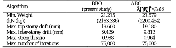
The section designations obtained by BBO algorithm to determine the optimum cold-formed steel frame design is tabulated in Table 1. In Table 2, minimum frame weight located by the BBO algorithm is compared with the available results reported in the literature based on an artificial bee colony (ABC) (Çarbaş  2013) algorithm for comparison purpose. The minimum weight for the cold-formed steel frame is obtained as 21.215 kN (2163.336 kg).The optimum design weight located by BBO algorithm is lighter than the design weight obtained by the ABC technique.

Table 2.Maximum constraintvaluesand minimum frameweightsfor 106-member industrialbuildingwithdifferentmetaheuristictechniques

Algorithm BBO

(present study)

ABC

(Çarbaş 2013)

Min. Weight (kN (kg))

21.215 (2163.336)

21.579 (2200.454) Max. top storey drift (mm) 19.660 19.180 Max. inter-storey drift (mm) 9.429 9.812 Max. strength ratio 0.988 0.964 Max. number of iterations 75,000 75,000

It is apparent from design example that in optimum design problem where the number of design variables relatively large, BBO algorithm worked efficiently without any problem. The maximum strength ratio, the maximum top storey drift and the maximum inter-storey drift values are 0.988, 19.660 mm and 9.429 mm, respectively. From these results, it can be concluded that the all constraints are almost at their upper bounds and both displacement and strength constraints are dominant in the optimization process.

V. CONCLUSION

REFERENCES

[1] A., Ghersi, R., Landolfo and F.M., Mazzolani, (2005). “Design of Metallic Cold-Formed Thin-Walled Members”, Spon Press, ISBN-13: 978-0415244374.

[2] Ad Hoc Committee on Serviceability, (1986). “StructuralServiceability: A Critical AppraisalandResearchNeeds.”Journal of StructuralEngineering, vol. 112(12), pp. 2646–2664.

[3] AISC (American Institute of Steel Construction), (1991). “LRFD, Volume 1, Structural Members, Specifications & Code”, Manual of Steel Construction, New York, U.S.A.

[4] AISI (American Iron and Steel), (2002). “Cold-Formed Steel Design Manual”, Milwaukee Wisconsin, U.S.A.

[5] AISI (American Iron and Steel Institute S100-07), (2007). “North American Specification for the Design of Cold-Formed Steel Structural Members.”

[6] AISI (AmericanIronand Steel Institute D100-08), (2008). “Excerpts-GrossSectionPropertyTables”, Cold-Formed Steel Design Manual, Part I; DimensionsandProperties.

[7] C.A.C., Coello, (2002). “Theoretical and numerical constraint-handling techniques used with evolutionary algorithms: a survey of the state of the art.”Comput Methods ApplMech, ,vol. 191, pp. 1245–1287.

[8] D., Simon, (2008). “Biogeography-based optimization.”IEEE Trans EvolutComput, vol.12(6), pp. 702–713.

[9] I., Boussaid, A., Chatterjee, P., Siarry, and M., Ahmed-Nacer, (2012). “Biogeography-based optimization for constrained optimization problems.” ComputOper Res, vol. 39(12), pp. 3293–3304.

[10] M.P., Saka et al., (2015). “Comparative study on recent metaheuristic algorithms in design optimization of cold-formed steel structures.” Chapter 9 of Engineering and applied sciences optimization. Springer, Switzerland, ISBN: 978-3-319-18319-0, pp. 145–173.

[11] M.P., Saka, S. Çarbaş,I., Aydoğdu, and A., Akın, (2016). “Use of Swarm Intelligence in Structural Steel Design Optimization.” Chapter 3 of Metaheuristics and Optimization in Civil Engineering, Springer, ISBN: 978-3-319-26245-1, pp. 43-73.

[12] O., Hasançebi, S., Çarbaş, E., Doğan,  F.,  Erdal, and  M.P., Saka, (2009). “Performance evaluation of metaheuristic search techniques in the optimum design of real size pin jointed structures.”ComputStruct, vol. 38(5-6), pp. 284-302.

[13] O., Hasançebi, S., Çarbaş, E., Doğan, F., Erdal, and M.P., Saka, (2010). “Comparison of non-deterministic search techniques in the optimum design of real size steel frames.”Computers & Structures, vol. 88(17-18), pp. 1033-1048.

[14] P.K., Ammu, K.C., Sivakumar, and R., Rejimoan, (2013).”Biogeography-based Optimization-A survey”, Int J Elect ComputScieEng, vol. 2,pp. 154-160.

[15] S.,  Çarbaş,  (2013). “Optimum Design of Low-Rise Steel Frames Made of Cold-Formed Thin-Walled Steel Sections”, Ph.D. Dissertation, Middle East Technical University, Ankara, Turkey.

[16] S., Kima, J., Byeonb, H., Yuc, and H., Liud, (2014). “Biogeography-based optimization for optimal job scheduling in cloud computing.”Appl Math Comput, vol. 247, pp. 266–280.

[17] S., Rajasomashekar and P., Aravindhababu, (2012). “Biogeography based optimization technique for best compromise solution of economic emission dispatch.”Swarm EvolComput, vol. 7, pp. 47–57.

[18] W-W., Yu and R.A., LaBoube, (2010). “Cold-Formed Steel Design, Fourth Edition.” John Wiley, ISBN: 978-0-470-46245-4.

[19] www.greenmaltese.com/2012/08/cold-formed-steel/, retrieved on 06.03.2016.