Instantaneous multiple input finite buffer system

Buffer System

Bih-Wang Lee

Arne

A.

Nilsson

Center for Communications and Signal Procesing

Department of Electrical and Computer Engineering

North Carolina State University

TR-90/6

Bih-Hwang Lee

Arne A. Nilsson

Center for Communications and Signal Processing

Department of Electrical and Computer Engineering

North Carolina State University

Raleigh, NC 27695-7914

(Phone): 919-737-3015

(FAX): 919-737-7382

ABSTRACT

A buffer is needed to store the excess information if the transmission rate of a

transmitter is less than its input rate. In this paper, a finite buffer is analyzed with

instantaneous multiple input, which has a deterministic interarrival time and a generally

distributed message size; the main objectives are to minimize the loss of data, and to

maximize the utilization of the system. Three performance measures are used to achieve

those purposes: the probability distribution function of the buffer occupancy is used to

characterize the usage of the buffer; the probability distribution function of the amount of

loss is used to determine if the loss is acceptable; and the utilization of the system refers to

the need to make efficient use of transmission facilities. Analytical expressions are obtained

for these performance measures. An approximation is obtained and compared with results

1. INTRODUCTION

Recently, computer communication networks have been used very widely to exchange

information between two systems. Figure 1 shows a communication environmentinwhich many stations are connected to a communication network. If a local station wants to send a

message to a remote station, then a certain procedure is followed: the message must first go

to the source node, then the message travels through zero or more intermediate nodes and

arrives at the destination node; fmally, the remote station receives the message.

Basically, the communication environment consists of three major systems: the source

system, the transmission medium, and the destination system. Depending upon the

functions of each element, we summarize the systems in Figure 2, e.g., a local station

functions as an input device, a source node functions as a transmitter, and the intermediate

nodes function as a transmission medium, etc.

The input device can be a computer, a data generator, or any data handling machine. If

the input device is an image coder, the image information is manipulated into a series of

digitaldata by the coder, and then the transmitter sends the data to the transmission medium upon receiving the data. The transmitter can immediately send data if its transmission rate is

greater than its input rate. Unfortunately, the transmission rate of a transmitter is often less

than the output rate of an input device, potentially resulting in a loss of data.

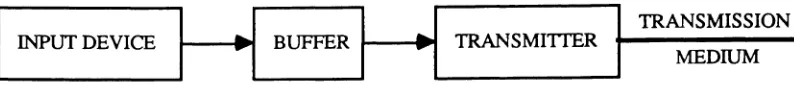
In order to prevent this data loss, we need a buffer in which the excess input to the

transmitter is temporarily stored, Figure 3. An interesting question is how large a buffer we

need. Of course, there is no loss if we have an infinite buffer, but this is very inefficient

and totally unrealistic. We also know that if the buffer is small, the loss can be considerable

unless we accept a reduction in the output rate of the input device; however, this reduction

implies a degraded performance. Generally speaking, if the buffer size increases, then the

cost increases, but the loss decreases. The main objectives of this research are to minimize

the loss and to maximize the utilization of the system.

The performance of the buffered system can be evaluated by obtaining the probability

distribution function of the buffer occupancy, the probability distribution function of the

amount of loss, and the utilization of the system. From the probability distribution function

of the buffer occupancy, we know how the buffer has been used. Furthermore, we use the

probability distribution function of the amount of loss to determineifthe loss is acceptable. The utilization of the system refers to the need to make efficient use of transmission

loss is relatively small or acceptable, i.e., the probability that the buffer is empty should be

small, and the probability of no loss should be relatively high.

Remote stations

Transmission

----+---

Destination system

medium Intermediate nodes

Source system

----+---Localstations

Figure 1 A communication environment

INPUT

DEVICE

TRANSMITTER TRANSMISSION

MEDIUM RECEIVER

OUTPUT

DEVICE

~_~----

_...V-

- - - - , . , . , )

Source system Destination system

I

rnPUT DEVICE

I 1

BUFFER

I

Figure 3 A buffered source system.

2. Description

1

TRANSMITIER

I

TRANSMISSION

MEDIUM

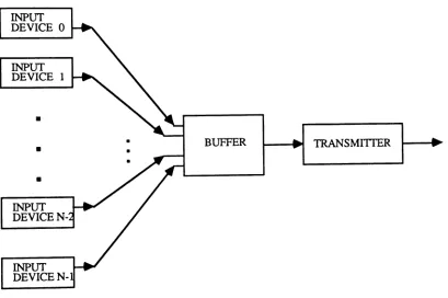
We assume that there is a total of N input devices connected to a common buffer,

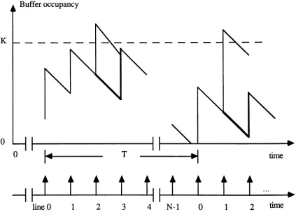
Figure 4; these input devices are scheduled alternately to send a message within a time slot, which is a fixed time interval T. We also divide a time slot into N pieces, called time shiftt

( 't =TIN ).After a time shift, another input line starts its own time slot to begin sending its message, i.e., the time slot of the next line lags by time t. In other words, if the time slot of line 0 begins with time 0, then, in turn in round robin fashion, the time slot of the next line begins with timet; the others begin with time2t,3't, ...,(N-l)t,etc. At time T, line 0

again obtains its own time slot to send the remaining part of the message; however, any

message can be sent only at the beginning of its own time slot. We assume that the

message size which can be brought into the buffer in a time slot is generally distributed; the

probability distribution function of the message size is denoted by Bi(X), and its density function is bi(x), where i=O, 1, ...,N-l. We also assume that the propagation delay from

each input device to the buffer is the same as the others; otherwise, the time shift in our

analysis is no longer a constant. Any input line may use several consecutive time slots, a

busy-period, to send an entire message; then it remains in idle status for some time, an

idle-period. We assume that the busy-period and the idle-period are geometrically distributed.

If the buffer is empty at the time when any message enters, then the message is

transmitted through the medium immediately; however, if the input rate of the buffer is

greater than its output rate, the excess message has to be stored in the buffer. In this paper,

we assume that the output rate of the input devices is much greater than the transmission

rate of the transmitter, i.e., an instantaneous input. When no message arrives and the

buffer is not empty, the messages are still transmitted until the buffer becomes empty; that

is, the system is entirely idle. The queueing model for this system is shown inFigure 5. Since the buffer size is finite, any message in excess of the capacity of the buffer, K,

is lost. However, in this system, not only is the excess message destroyed, but also the

entire message brought into the buffer at the time slot is destroyed as well. Because a

the trailer of the message; hence, the header and the trailer cannot be ignored. In data

communication, a message must contain several kinds of information, such as routing and

error controls, for transmitting data from a source system to another destination system.

The buffer occupancy with timing for each line is shown in Figure 6. Note that the lost

message could be re-sent, depending on the protocol of the source system, which we do

not discuss here. However,ifa lost message could be re-sent, we would still count the lost

message as a loss in our system. On the whole, this is a very complicated, but realistic,

system.

INPUT DEVICE 0

INPUT DEVICE 1

•

•

•

INPUT

DEVICEN-INPUT

DEVICEN-BUFFER TRANSMfITER

line 0

line 1

line N-2

line N-I

Periodic input

~'---"" ~---')

_V

Finite buffer

Figure 5 A [mite buffer queueing model with multiple inputs.

Buffer occupancy

time

2

1

o

--~

t

t

t~

T

I~

o

----1

~t

t t t

~ ~t

line0 1 2 3 4 N-1

K

o

3. Analysis

In order to analyze the system, we use an embedded Markov chain analysis. The

embedded points are chosen to be the input time at which a new message has not been

entered. We need to consider not only the probability distribution functions of the busy and

idle periods, but also the probability distribution function of the message size sent at the

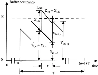
beginning of the time slot. A detailed Markov chain description is shown in Figure 7.

Buffer occupancy

loss

K

,

Yi+1,n

I ~

(n+1) T

time

T

o

Figure 7 The embedded Markov chain description for multiple input lines.

LetYi,n and Xi,nrepresent the buffer occupancy before a new message enters at time

slot n of line i, and the message size entering from line i to the buffer at time slot n of line i,

respectively. A loss occurs if any part of a message exceeds the capacity of the buffer. The amount of loss at time slot n of line i is denoted by Zi,n' where n= 0,1,2, .... , and i = 0,

1, ..., N-1. The units are in bits for all variables mentioned above; both time slot T and time shift t are in seconds. For simplicity, we assume that the transmission rate of the

, +

Yi+_1,n

=

[Yi,n - t] (1)

where [x]" = max [0, x] and

and

Yi,n line i is idle at time slot n

line i is busy at time slot n, and overflow occurs

line i is busy at time slot n, and no overflow occurs.

~,n

= {

o

elsewhere. ₍₂₎

Based upon the embedded Markov chain description, we analytically, by definition,

obtain an integral equation for the probability distribution function of the buffer occupancy

and equations for the probability distribution function of the amount of loss and for the

utilization of the system.

3.1. The Probability Distribution Function of The Buffer Occupancy

According to the definition of Yi,n' we know that the value of Yi.nis never more than Kvt; hence, the probability distribution function of the buffer occupancy must be equal to

one for y ~ K-t. We let Wi,n(y) represent the probability distribution function of Yi,n.

Consequently, we only need to consider the case of y

<

K-t; by definition, we have

Wi+1,n(y) = Pr{Yi+1,n

s

y)

=Pr{Y:,n

s

y

+

t}

=

Pr{y'i,n ~y+t I line i is busy) Pr{line i is busy) +

Pr{Y'i.n

s

y+tIline i is idle} Pr{line i is idle}. (3)

However, we are only interested in the stationary distribution function of Wi,n(y), which is

denoted by Wi(y); by definition, we have

Wi(y) = 1 i m Wi,n(Y) .

We assume that the limit exists and that the limiting distribution is independent of theinitial

state Yi,o; hence, Wi(y) is the stationary probability distribution function of the buffer

occupancy at the time slot of line i, and its density function is wi(y). Similarly, for

long-term behavior, we use Y, for the buffer occupancy at the beginning of the time Sl9t of line i

and Xi for the message size to be brought into the buffer by line i. Furthermore, let BPi and IP_ibe the proportions of the expected values of the busy-period and the idle-period of

line i, respectively. If the busy-period is geometrically distributed with parameter Pi' then

its expected value is l/Pi; similarly,with parameter qi for the idle-period, the expected

value is l/qi. Hence, we have

l/Pi

Bp·

=

and

II/Pi

+

l/qi l/Cli

I p · = -II/Pi

+

l/Cli

(5)

(6)

Since we are considering the long-term behavior of the system, for convenience, we use

BPi for Pr{line i is busy} and IP_i for Pr{line i is idle} through this paper. Therefore, we

obtain W_i+₁(y) as follows:

W_i+1(y)= Pr {y\

s

y+'t Iline i is busy} BPi +Pr {Y\

s

y+t Iline i is idle} IPi (7)

We assume that the stationary probability distribution function of the buffer occupancy is

continuous in [0, Kvt], and that Wi(O)

~

0; hence, we have Wi(O+) ,., Wi(O) and wi(O)

=

Wi(O) o(y). We consider two cases ( 0

s

y <K-2t and K-2t

s

Y<K-t ) to obtain the probability distribution function of the buffer occupancy.

Case 2: K-2t

s

y < K-t

Wi+_1(y) = Pr{Y'i

s

y+t Iline i is busy} BPi + Pr{Y'i

s

y+t I_{line i is idle} IPi}

=

{foK--'tWi(X) Bi(y+t-x)dx + foK--'tWi(X) [l-Bi(K-x)] dx}BPi + IP_i

={

_{Bi(y+2t-K)+foK--'tWi(X) bi(y+t-x)}dx - Bi(t) - foK--'tWi(X) bi(K-x)dx }BPi + 1

3.2. The Probability Distribution Function of The Amount of Loss

(9)

Let Li,n(z) denote the probability distribution function of the amount of loss at time

slot n of line i; by definition Li,n(z) = Pr{Zi,n~ z}. Again, we are interested in the

stationary distribution function of Li,n(z), which is denoted by Li(z); by definition,

Li(z) = lim Li,n(z) .

n ~ 00 (10)

This limiting distribution must exist and is independent of the initial state ~,o; hence, Li(z)

is the stationary probability distribution function of the amount of loss at the time slot of line i. Similarly, for long-term behavior, we use ~for the amount of loss at the time slot of

line i. In order to obtain Li(z), let us first determine its probability density function in the

busy period, which is denoted by li(x). According to the criteria of the loss measure when

we only accept the whole message, the amount of loss is, obviously, either equal to zero or greater than t; hence, we summarize li(X) as follows:

li(X)

=

Pr{loss

=

xIline i is busy}

Bi(t) +

L

K

bi(x) WiCK-x) dx for x=O

0 for O<x~t

=

bi(x) [1-Wi(K-x)] for t<x~K

bi(x) for x>K

(11)

(12) for z>K

for t <Z~K

for 0

s

z

s

t

B·(z) BP·_{I I}

+

IP·_I

=

=

foz

li(x) dx BPi + IP j

[ Bj('t) +

l

K

bj(x) WiCK-x)dx] BP j + IP_i

[ Bj(z) +

L

K

bj(x) Wj(K-x)dx] BP j + IP j

3.3. The Utilization of The System, P

By definition, we have the utilization at the time slot of linei as follows:

pj = BPj

[f f

Pr{Xj= x and

v,

= YI x+y

s

K and x-t-y

~

d

dydx

+

ff

Pr{Xj

=

x and

v,=

YI x-l-y

~

K and x+y <

d

x:

y dydx

+

ff

Pr{Xj = x and Yj= YI x--y>K and y

~

d

dy dx

+

ff

Pr{Xj

=

x and Yj

=

YI x+y

>

K and y<r}

~

dydx]

+ IPj

[f

Pr{Yj

=

YIY

~

't} dy +

f

Pr{Yj

=

YIY<

d

~

dy]

(13)

and the utilization of the system,

p,

is determined as:

N-l

p=

~

LPj

i=O (14)

We consider two cases (K-t 2:t and K-t<t ) to obtain

= 1 -

1.

E[idle period of line i]

~

Furthermore, E[idleperiod of line i] can also be, by defmition, obtained, i.e.,

E[idle period of line i]

=

BPi

[JJ

Pr{X_i

=

x andY_i

=

YIx+YSK and x+Y<

tl

(-r-x-y) dy dx

+

JJ

Pr{X_i

=

x andY_i

=

YIx--y>K and y

<

tl

(-r-y) dy dx]

+ IP_i

J

Pr{Y_i

=

Y I y<-r} (-r-y) dy

Case2: K·~ < ~

(15)

(16)

Pi

=

1 -

~

{ -r - LK-'ty Wi(y) dy + BPi

[L

2

1:- KBi(x)dx _{+ [B i(2-r-K)-Bi(K)]f:-'tWi(y) dy}

+

J1:

bi(x)

r1:-X

Wi(y) dy

dx -

(2-r- K) Bi(-r) + (K --r)lK Wi(K-x) bi(x)

dx

~K

k

~

-l

Kx

Wi(K-x) bi(x)

dx

+

l

K

bi(x)

J:":

Wi(y) dy

dx]}

=

1 -

1.

Elidleperiod of line i]

~ (17)

4. Approximation for Erlang Distributed Data Input

We have obtained the integral equation for the probability distribution function of the buffer occupancy, and the equations for the probability distribution function of the amount of loss and for the utilization of the system; however, we cannot solve for them because the message size is generally distributed. In this section, we choose an Erlang distribution for the message size and attempt to solve the equations.

Itis verydifficult to find an analytical solution for the integral equations of (8) and (9). We have, however, obtained a polynomial approximation as follows:

N

W i(y)

=

Ci,o +

I.

Ci,n yn

n=l

for N

=

3, 4, or 5 ,

(18)

The power series expansion for approximately solving the integral equation which we

have used here normally proceeds as we try to match coefficients for the power of, in this

case, y. Due to the complexity of the functions in the derivations, this approach is not feasible for our problem. We have instead adopted the least mean square error method to obtain the expression for the unknown coefficients

q,n'

n=0, 1, ... , N. By this method,

CL,i+lis the mean square error for solving Wj(y), where L is the number of points used to

make a higher accurate operation. Certainly a good approximation can be achieved by using

a large number for L. We find that it is sufficient to use the number 100 for L. In order to

minimize the error, we take the derivative ofCL,i+l with respect toCi+1,kfor k

=

0, 1, ...,

N, and set that derivative to zero. Lengthy manipulations give us an equation for the coefficients ( Ci+_{1,O, Ci}+_{1,1, · .. ,} Ci+1,N ). Note that we have the boundary condition to make N+l linear independent equations to solve for the N+l Ci,n's for each line. After

finding Wi(y), then Li(z) and Pi can be analytically obtained. Note also that we have

considered Wj(Y) for two cases; hence, this approximation should alsobediscussed in this manner.

5. Example

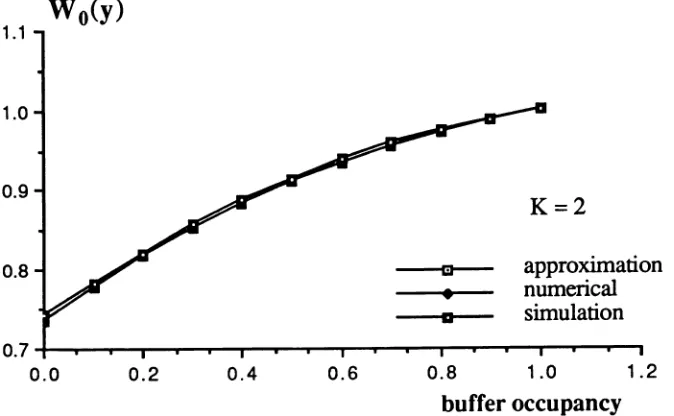
Inthis section we show through some results that the approximate solutions for Wi(Y) and Lj(z) are very accurate, which is demonstrated by comparing the results obtained from

the approximate analysis, a numerical method, and a simulation experiment. The case

which we have used for comparison has an Erlang-2 distributed message size, three input lines, and the additional parameters Jl

=

1.1, T

=

1, and K

=

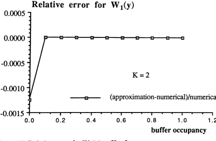
2. Figures 8 to 15 show the results and the relative errors for Wj(Y) and Lj(z), where i= 0 and 1. We omit the results

for line 2 because they are very similar to the other lines. The results obtained from these

three approaches are very close; therefore, we use a relative error to show how close the

results obtained are from the approximation and the numerical method. The maximum

relative errors are less than 0.2% and 0.11% for W(y) and L(z), respectively. We have

found that if N

=

4, then the approximate results are very close to the results obtained from

the other two approaches. Clearly, increasing N increases the accuracy of the polynomial

Wo(y)

1.1

1.0

0.9

0.8 m

•

a

K=2

approximation numerical simulation

0.6

0.4 0.2

o.

7-+---.-...---.~...-...-...-...--.---...~~...--...--...---r---.---,

0.0 0.8 1.0 1.2

buffer occupancy

Figure 8 Wo(Y)obtained from the three approaches as K

=

2.

Relative error for W

o(Y)

0.001

0.000

-0.001

(approximation-numerical)/numerical

0.8 1.0 1.2

butTer occupancy

0.6

0.4 0.2

-0.002 -+---r-~---r---,r--~...,...---r---r---.-...-....-...-...-.-....--.

0.0

1.1

1.0

0.9

0.8

•

a

K=2

approximation numerical simulation

0.6 0.4

0.2

O. 7-t-"-r---.---,.-..-r---r--.,...-...,....-....---r---._...--....-~...---.-...

0.0 _{0.8 1.0 1.2}

buffer occupancy

Figure 10 Wt(y) obtained from the three approaches as K

=

2.

Relative error for W

1(y)

0.0005

0.0000

-0.0005

-0.0010

K=2

m (approximation-numerical)/numerical

-0.0015

0.0 0.2 0.4 0.6 0.8 1.0 1.2

buffer occupancy

Lo(z)

0.960

0.958

0.956

a

0.954

•

a

0.952

0.950

0.948

0.946 0

K=2

approximation numerical simulation

2

amount of loss

Figure 12 Lo(z) obtained from the three approaches as K

=

2.

Relative error for Lo(z)

K=2

a (approximation-numerical)/numerical

1.5 2.0

amount of loss

1.0

0.5

-1 -r--r-r-r--"'I--..--r--r--,--r--r-~r---t--..--,---.-...-r-....-~...--.--.

0.0

0.954

approximation numerical simulation

a

l!I

•

K=2

0.942-4---e-B~

0.944 0.946 0.948 0.950 0.952

2

0.940 - , - - - . , . . - - - . . - - - . . - - - .

o

amount of loss

Figure 14 L1(z) obtained from the three approaches as K=2.

Relative error for L

_1(z)

0.0012

0.0010 m

0.0008

0.0006

0.0004

0.0002

0.0000 0

(approximation-numerical)/numerical .

K=2

2

amount of loss

6. Conclusion

In this paper we present solutions to the performance analysis of the finite buffer

system with instantaneous multiple input. An integral equation is derived for the probability

distribution function of the buffer occupancy at the beginning of an input message

generation; equations are also derived for the utilization of the system and the probability

distribution function of the amount of loss due to the overflow of the finite buffer. It is

shown that a very accurate polynomial approximation does exist. The accuracy of this

approximation is compared with the result obtained from a numerical solution of the

integral equation, as well as the result obtained from the simulation experiment. The main

advantages of the approximation are the accuracy and the reduction in computational