Development of Geomorphological
Instantaneous Unit Hydrograph – A Case
Study of Hemavathi Catchment
Ashwini B1, Mamatha2
Assistant Professor, Department of Civil Engineering, PES College of Engineering, Mandya, Karnataka, India1
Research Scholar, DOS in Earth Science, University of Mysore, Karnataka, India2
ABSTRACT:Geomorphological Instantaneous Unit Hydrograph (GIUH) model which proves to be simple and analytical approach is popular because of its direct application for proper assessment of runoff response to an ungauged catchment resulting from a rainfall event. It is an essential for protection of environment issues for sustainable development of life and hydrological response of Hemavathi catchment. It avoids adoption of tedious methods of regionalization of unit hydrograph where in, the historical rainfall – runoff data are required to be analysed. In this study, the GIUH based Nash model has been developed for the estimation of direct surface runoff hydrographs. The GIUH derived from geomorphological characteristics of Hemavathi catchment has been related to the parameters of Nash model for deriving its complete shape in which these shape parameters of the Nash model is found to depend on Horton’s ratios of area ratio (Ra), bifurcation ratio (Rb) and length ratio (Rl) of the catchment and thus obtained GIUH
is compared with the CWC method of unit hydrograph.
KEYWORDS:GIUH, Nash model, CWC method of unit hydrograph
I. INTRODUCTION
I.I.Background of GIUH Based Approach
Rodriguez-Iturbeand Valdes (1979) introduced the GIUH model to assess the direct runoff of catchment and theory of relating the peak discharge and time to peak discharge with geomorphologic characteristics of the catchment and a dynamic velocity parameter. Thsi Pioneer work of Rodriguez-Iturbe and Valdes which explicitly integrates the geomorphologic details and the climatologic characteristics of the basin which is a framework of travel time distribution which is boon for stream flow synthesis in the basin having no or scanty information of flow data. This formulation of GIUH is based on the probability density function (pdf) of the time history of a randomly chosen drop of effective rainfall arrived to the trapping state of a hypothetical basin, treated as a continuous Markovian process, where the state is the order of the stream in which the drop is located at any time and the value of this pdf produces the main characteristics of GIUH.
qp = 1.31 Rl0.43 V/ L (1)
tp = 0.44 (L /V) (Rb/Ra)0.55χ Rl-0.38 (2)
Where, qpis the peak flow, L is the length of the highest order stream (km), V is the dynamic velocity parameter (m/s). Multiplying equations (1) and (2) a non-dimensional term qp χ tp is derived as.
qp χ tp = 0.5764 [ Rb / Ra ] 0.55χ Rl0.05 (3)
of climatic variation. Rodrigluez-Iturbe et al. (1979) showed the dynamic velocity parameter of the GIUH can be taken as the velocity at the peak discharge time for a given rainfall-runoff event in the catchment. Valdes et.al. (1979) compared the GIUHs for some real world basin with the IUHs derived from the discharge hydrograph predicted by a physically based rainfall- runoff model of the same basins and found them to be remarkably similar. For few of Indian catchments this GIUH based approach was successfully demonstrated (Kumar et.al. 2002; 2007). In the present study, the Nash based model was tested for the Hemavathi catchment.
I.II. NASH Model
The Nash model (Nash, 1957) is based on the concept of routing of the instantaneous inflow through a cascade of linear reservoirs with equal storage coefficient. The Nash model can be expressed as follows:
u (t) = (t/k) n-1 ( ) (4)
Where u (t) is the ordinates of IUH (hour-1), t is the sampling time interval (hour), n and k are the parameters of the Nash model, in which n is the number of linear reservoirs, and k is the storage Coefficient (hour).
The complete shape of the GIUH can be obtained by linking the qp and tp of the GIUH with scale (k) and shape (n) parameters of the Nash model. By equating the first derivative with respect to t of eq (4) to zero, t becomes the time to peak discharge, tp. Thus, taking the natural logarithm of both sides of eq (4), differentiating with respect to t and by simplification eq. (5) is derived.
ln [u(t)] = - + ( ) (5)
Equating eq. (5) to zero results in by replacing t with tp,
t= tp= k (n-1) (6)
Simplifying the value of tp from equation (6) in equation (4) and simplifying yields qp = [ ( )]χ (n-1)(n-1) (7)
Combining equations (6) and (7) results: qpχtp =
( ) [ ( )]
χ (n-1) (n-1) (8)
Equating equation (8) with equation (3) results in:
( ) [ ( )]
χ (n-1) (n-1) = 0.5764[Rb / Ra] 0.55 χRl0.05 (9)
The Nash parameter n, can be obtained by solving equation (9) using the Newton-Raphson method. The Nash’s parameter k for the given velocity V is obtained using equation (2) and (6) and the known value of the parameter n as follows:
k = . [Rb / Ra] 0.55χRl -0.38 ( ) (10)
The derived values of n and k are used to determine the complete shape of the Nash based GIUH using equation (4).In this paper GUIH based NASH model Geomorphological parameters have been estimated using GIS, since the use of GIS not only make this task relatively easy but accurate as well with the following objectives. 1) Development of Geomorphological Instantaneous Unit Hydrograph. 2) To validate the model using CWC method of unit hydrograph.
II. STUDYAREA
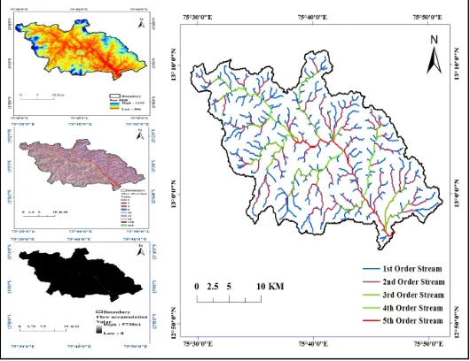
Fig1. Location Map of Hemavathi catchment
of Hemavathi catchment which is geographically lies between 12º50' 0" and 13º10' 0" North latitude and 75º 30 '0" and 75º 50' 0" East in south western part of Chickmagalur and Hassan districts as shown in figure 1.
III.MATERIALSANDMETHODOLOGY
To estimate the geomorphological parameter of the study area the catchment is delineated using ASTER Global DEM (Digital elevation model) of 30 m resolution which is downloaded from USGS earth explorer which represents the digital topographical surface using ArcGIS 10.3 software.
The study was carried out in two phases:
1. Extraction of drainage networks form the DEM using the flow direction method, which consists of the following steps (O’Callaghan and Mark, 1984).
a. Fill sinks: A sink is an uncompleted value lower than the values of its neighbourhood. To ensure proper drainage mapping, these sinks were filled by increasing elevations of sink points to their lowest outflow point.
b. Calculate Flow Direction: using the filled DEM produced in the step (a) the flow directions were calculated using the eight-direction flow model, which assigns flow from each grid cell to one of its eight adjacent cells in the direction with the steepest downward slope.
c. Calculate Flow Accumulation: Using the output flow direction raster created in step (b) the number of upslope cells flowing to a location was computed.
d. Stream Segmentation: After the extraction of drainage networks, a unique value was given for each section of the network associated with a flow direction.
e. Define Stream Network: The next step is to determine a critical support area that defines the minimum drainage area that is required to imitate a channel using a threshold value.
f. Morphometric Analysis using Strahler’s classification method (Strahler, 1964).
2. Development of GIUH model: To develop GIUH model the parameters obtained from the morphometric analysis
has been used in the present study which was first introduced by Rodriguez-Iturbe and Valdes (1979) and to develop complete hydrograph Nash model is used.
IV. RESULTS AND DISCUSSIONS
The quantitative morphometric analysis of the drainage basin is considered to be the most satisfactory method because it enables us:
i. To understand the relationship between different aspects of the drainage pattern of the same drainage basin. ii. For comparative evaluation of different drainage basins developed in various geologic and climatic regimes. iii. To define certain useful parameters of drainage basins in numerical terms.
Remote sensing and Geographic Information System (GIS) techniques are being efficiently used in recent times as a tool in determining the quantitative description of basin geometry that is morphometric analysis also people have developed unit hydrograph also.
In this output map totally 5 orders are identified. Total number of 1st order streams is 316 with length 283.55km, total number of 2nd order streams is 72 with length 116.77km, total number of 3rd order streams 17 with length in 83.4km, total number of 4th order streams 4 with length 31.71km, and the total number of 5th order streams 1 having length 27.17 km which is shown in figure 2 also Horton’s ratios are found to be Bifurcation ratio (Rb) is 3.38, Length ratio (Rl)
is 1.98 and Stream-area ratio (Ra) is 0.465.
Fig 2. Stream order map of Hemavathi Catchment
The drainage pattern of the basin is predominantly dendritic and semi-dendritic pattern is less pronounced. The types of drainage patterns indicate lack of inhomogeneity in the geological formation and structural control. The quantitative morphometric analysis coupled with limited field studies demonstrate the hydrological nature of the underlying geology, precipitation, exogenic and endogenic forces operating within the basin [15].
IV.I. Estimation of Geomorphological Instantaneous Unit Hydrograph
The final form of the GIUH is obtained by substituting the value of Ra, Rb, Rland value of k at different dynamic
Table 1. Value of k at different dynamic velocity
V (m/s) n k V(m/s) n k
0.50 3.9 18.9341 3.00 3.9 3.1556
1.00 3.9 9.467 3.50 3.9 2.7048
1.50 3.9 6.311 4.00 3.9 2.3667
2.00 3.9 4.7335 4.50 3.9 2.1037
2.50 3.9 3.7868 5.00 3.9 1.893
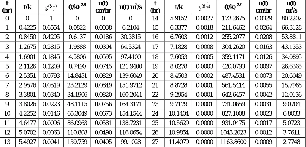
Table 2. Derivation of Nash based unit hydrograph at dynamic velocity 4 m/s, k = 2.3667 and n = 3.9 is as follows
t
(hr) t/k ( ) (t/k)
2.9 u(t)
cm/hr u(t) m
3
/s t
(hr) t/k ( ) (t/k)
2.9 u(t)
cm/hr
u(t) m3/s
0 0 1 0 0 0 14 5.9152 0.0027 173.2675 0.0329 80.2202
1 0.4225 0.6554 0.0822 0.0038 6.2104 15 6.3377 0.0018 211.6462 0.0264 66.3128
2 0.8450 0.4295 0.6137 0.0186 30.3815 16 6.7603 0.0012 255.2077 0.0208 53.8811
3 1.2675 0.2815 1.9888 0.0394 64.5324 17 7.1828 0.0008 304.2620 0.0163 43.1353
4 1.6901 0.1845 4.5806 0.0595 97.4100 18 7.6053 0.0005 359.1171 0.0126 34.0895
5 2.1126 0.1209 8.7490 0.0745 121.9400 19 8.0278 0.0003 420.0793 0.0097 26.6365
6 2.5351 0.0793 14.8451 0.0829 139.6049 20 8.4503 0.0002 487.4531 0.0073 20.6049
7 2.9576 0.0519 23.2129 0.0849 151.9712 21 8.8728 0.0001 561.5414 0.0055 15.7968
8 3.3801 0.0340 34.1906 0.0820 160.2041 22 9.2954 0.0001 642.6457 0.0042 12.0136
9 3.8026 0.0223 48.1115 0.0756 164.3171 23 9.7179 0.0001 731.0659 0.0031 9.0704
10 4.2252 0.0146 65.3049 0.0673 154.1544 24 10.1404 0.0000 827.1008 0.0023 6.8033
11 4.6477 0.0096 86.0963 0.0581 138.7231 25 10.5629 0.0000 931.0475 0.0017 5.0723
12 5.0702 0.0063 110.808 0.0490 116.0654 26 10.9854 0.0000 1043.2023 0.0012 3.7611
13 5.4927 0.0041 139.759 0.0405 99.1028 27 11.4079 0.0000 1163.8600 0.0009 2.7748
We tried to derive Complete Derivation of Nash based unit hydrograph at velocities and by trial and error we got 4 m/s is found to be good, therefore here we described only at 4m/s (Table 2) according to the procedure given by Rodriguez-Iturbeand Valdes (1979) which is already described in I.I and I.II.
IV.II. Validation of GIUH with CWC Method of Unit Hydrograph
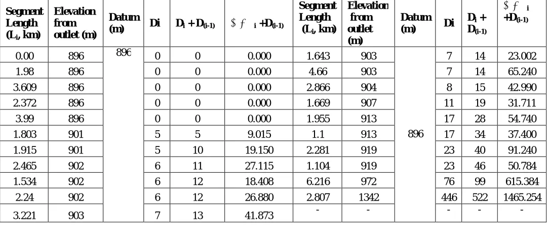
Table 3. Calculation of slope
Segment Length (Li, km)
Elevation from outlet (m)
Datum
(m) Di Di + D(i-1) L χ Di +D(i-1)
Segment Length (Li, km)
Elevation from outlet (m)
Datum
(m) Di
Di +
D(i-1)
L χ Di
+D(i-1)
0.00 896 896 0 0 0.000 1.643 903
896
7 14 23.002
1.98 896 0 0 0.000 4.66 903 7 14 65.240
3.609 896 0 0 0.000 2.866 904 8 15 42.990
2.372 896 0 0 0.000 1.669 907 11 19 31.711
3.99 896 0 0 0.000 1.955 913 17 28 54.740
1.803 901 5 5 9.015 1.1 913 17 34 37.400
1.915 901 5 10 19.150 2.281 919 23 40 91.240
2.465 902 6 11 27.115 1.104 919 23 46 50.784
1.534 902 6 12 18.408 6.216 972 76 99 615.384
2.24 902 6 12 26.880 2.807 1342 446 522 1465.254
3.221 903 7 13 41.873 - - - - -
∑LI Χ DI+D(I-1)=2620.186
S = 2620.186/ (51.43)2 = 0.99 m/km
The following information is obtained from the map of the Hemavathi catchment using ArcGIS.Catchment area as 589.15km2, Length of longest stream as 51.43 km, length of the longest stream nearest to Cg which is nothing but Lc as 22.64 km.Calculation of slope and other parameters are tabulated in table 3, further the parameters of CWC procedure of unit hydrograph described in table 4.
Table 4. Parameters of Unit Hydrograph Using CWC Method for Hemavathi Catchment
qp(m3/s/sq.km) 2.043/(Tp)0.872 0.2825
Tp(hr) 0.553(L χ Lc√S)0.405 9.669
W50 2.197/(qp)1.067 8.464
W75 1.325/(qp)1.088 5.242
WR50 0.799/(qp)1.138 3.367
WR75 0.536/(qp)1.109 2.275
TB (hr) 5.08(Tp)0.733 26.80
Tm (hr) Tp + tr/2 10.168
Fig 3. GIUH at different velocities Fig4. CWC method of Unit Hydrograph
Here figure 3 represents unit hydrograph which drawn from the results of geomorphometric analysis with varying dynamic velocities from 0.5m/s to 5m/s further figure 4 represents CWC method of unit hydrograph which is plotted with the help of parameters which is described in above table.
V. CONCLUSION
We have described here an analytical geomorphological transfer function representing the theoretical distribution of hydraulic lengths in a river basin. This model is based on the assumption that the reduced lengths distributions in order k (Strahler order) are similar and represented by a Gamma law. The analytical geomorphological transfer function results from the convolution of these n Gamma laws (equations 6 and 7) n being the total Strahler order in the river basin. This theoretical result is an analytical function depending on n + 1 geomorphological parameters which are easily available by simply reading a map or analysing digital data (DEM for example). After explaining the approach to obtain this analytical function (equation 7), we have tested our theoretical model for another catchment. It possible to give a fairly accurate description of the morphological structure of the stream network in the river basin.
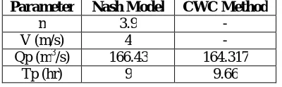
Table 5.Comparison of Nash Model with CWC method of unit hydrograph
Parameter Nash Model CWC Method
n 3.9 -
V (m/s) 4 -
Qp (m3/s) 166.43 164.317
Tp (hr) 9 9.66
From the present work Hemavathi catchment is found to be 5th order and almost steep terrain. Also, the extracted drainage network of the basin has wide range of application such as installation of the artificial drainage system and laying down the canal system, site identification for rain water harvesting, ground water recharge and waste disposal, etc. However the main theme of the study is to develop a GIUH. To check the accuracy of the GIUH technique the results were compared with CWC procedure of Unit hydrograph, three Horton’s ratios of the study areas were coupled with the parameters of Nash’s IUH model and the GIUH is derived for different values of dynamic velocity of flow. The results shows that the obtained GIUH with dynamic velocity 4m/s (approx.) for the catchment shows closer
0 50 100 150 200
0 5 10 15 20 25 30
V=0.5m/s V=1.0m/s
V=1.5m/s V=2.0m/s
V=2.5m/s V=3.0m/s
V=3.5m/s V=4.0m/s
V=4.5m/s V=5.0m/s
Time ((hr)
U
(t)
(m
3
/s
)
0 50 100 150 200
0 5 10 15 20 25 30
Time (hr)
U
H
(m
3/s
agreement with CWC approach (table 5). Since, CWC approach is independent of climatic parameter and geomorphologic characteristics other than the slope, drainage area and length of main stream resulting unit hydrograph may have some computational error.
REFERENCES
[1] Al-Wagdany, A. S., and Rao, A. R.., “Correlation of the velocity parameter of three geomorphological instantaneous unit hydrograph models.” Hydrol., Process. 12, 651-659, 1998.
[2] Aravinda, P.T., and Balakrishna, H.B.,”Morphometric analysis of vrishbhabathi watershed using remote sensing and GIS.”J. 2(8), 514-522, 2013. [3] Bhadra, A. Pnigrahi, N., Singh, R., Raghuwanshi, N. S., Mal, B. C., and Tripathi, M. P., “Development of geomorphological instantaneous unit hydrograph model for scantly gauged watersheds.” Environmental Modelling & Software, 23, 1013-1025, 2008.
[4] Bhaskar, N. R., parida, B. P., and Nayak, A. K., “Flood estimation for ungauged catchments using the GIUH.” J. Water Resour. Plng. and Mgmt., 12 (4), 228-238, 1997.
[5] Flood estimation report for cauvery basin subzone 3(i), central water commission New Delhi. 1986.
[6] Fleurant, C., Kartiwa, B., and Roland, B., “Analytical model for a geomorphological instantaneous unit hydrograph.”Hydrol. Process, 20, 3879-3895, 2006.
[7] Franchini, M and Connell, P.E., “An analysis of the dynamic component of the geomorphometric instantaneous unit hydrograph.”J. Hydrol. 175, 407-428, 1996.
[8] Gupta, V. K., Waymire, E., and Wang, C.T., “Representation of an instantaneous unit hydrograph from geomorphology.” Water Resources. 16(5), 855-862, 1980.
[9] Jain S. K., Singh, R. D., and Seth, S. M., “Design flood estimation using GIS supported GIUH approach.” Water Resour. Manage. 14, 369-376, 2000.
[10] Jain, V., and Sinha, R., “Derivation of unit hydrograph from GIUH analysis for a Himalayan river.” Water Resour. Manage. 17, 355-375, 2003. [11] Kirshen, D. M., and Bras, R.L., “The linear channel and its effect on the Geomorphologic IUH.” J. Hydrol. 65, 175-208, 1983.
[12] Kumar, R., Chatterjee, C., Lohani, A. K., Kumar, S., and Singh, R. D., “Sensitivity analysis of the GIUH based Clark model for a catchment.” Water Resour. Manage. 16, 263-278, 2002.
[13] Kumar, R., Chatterjee, C., Singh, R. D., Lohani, A. K., and Kumar, S., “Runoff estimation for an ungauged catchment using geomorphological instantaneous unit hydrograph (GIUH) model.”Hydrol. Process, 21, 1829-1840, 2007.
[14] MokarramMarzieh., and Amoorthy Santy Dinesh.., “Morphometric analysis of north fars watershed, Iran.”Journal of Geography. 6(4), 8-106, 2015.
[15]Mamatha, Janardhana. M., R2, Dinesh. A., “Quantitative Morphometric Analysis to Infer the Hydrological Behaviour of the East Suvarnamukhi basin in Tumkur district, Karnataka using Remote Sensing, GIS and bAd (bearing, Azimuth and drainage Calculator)”, International Journal of Innovative Research in Science, Engineering and Technology,Vol. 5, Issue 9, September 2016.
[16] ParetaKuldeep., and ParetaUpasana.,”Quantitative morphometric analysis of a watershed of Yamuna basin, India using Aster (DEM) data and GIS.” J. 2 (1), 248-269, 2011.