System reliability analyses and optimal maintenance planning of corroding pipelines

(1)

Scholarship@Western

Electronic Thesis and Dissertation Repository

7-18-2017 12:00 AM

System reliability analyses and optimal maintenance planning of

corroding pipelines

Changqing Gong

The University of Western Ontario Supervisor

Wenxing Zhou

The University of Western Ontario

Graduate Program in Civil and Environmental Engineering

A thesis submitted in partial fulfillment of the requirements for the degree in Doctor of Philosophy

Follow this and additional works at: https://ir.lib.uwo.ca/etd

Part of the Civil Engineering Commons

Recommended Citation Recommended Citation

Gong, Changqing, "System reliability analyses and optimal maintenance planning of corroding pipelines" (2017). Electronic Thesis and Dissertation Repository. 4669.

https://ir.lib.uwo.ca/etd/4669

This Dissertation/Thesis is brought to you for free and open access by Scholarship@Western. It has been accepted for inclusion in Electronic Thesis and Dissertation Repository by an authorized administrator of

(2)

i

The failure of corroding pipeline joints may induce severe consequences. However, maintenance is expensive due to the cost of excavating and repairing a single joint and typically a significant number of joints that need repair. It is central to develop an optimal cost-effective maintenance strategy that balances cost and safety. A key component of the strategy is the reliability based condition evaluation of pipeline joints. The focus of the research reported in this thesis is therefore developing efficient reliability assessment methods for pipeline individual joints, and developing an optimal maintenance framework for the entire pipeline system.

First, efficient system reliability methods relying on the first-order reliability method (FORM) and important sampling (IS) are developed for the assessment of the time-dependent probabilities of small leak and burst failure of pipeline joints containing multiple corrosion defects. In addition, a novel method is developed within the FORM to obtain the design points efficiently. An improved equivalent component approach for evaluating multi-normal integrals is also developed to improve the efficiency of the FORM for system reliability analysis.

In addition, a multi-objective optimization-based maintenance framework for corroding pipeline systems is formulated optimizing three objectives, i.e. the conditioned probabilities of burst and small leak, respectively, and repair cost. An improved genetic algorithm with a pre-training population is utilized to investigate the optimal Pareto front. The benefits of this framework enable decision makers to access a series of non-dominated optimal repairing solutions with respect to multiple conflicting objectives.

Keywords:

First Order Reliability Method, design point, multi-normal integral, small leak,

(3)

ii

Co-Authorship Statement

A version of Chapter 2, co- authored by Wenxing Zhou, Changqing Gong and Hanping Hong, has been published in Journal of Engineering Mechanics, ASCE, 2017, 143(9), DOI: 10.1061/(ASCE)EM.1943-7889.0001280

A version of Chapter 3, co- authored by Changqing Gong and Wenxing Zhou, has been published in Structural Safety, 2017, 68, 65-72

A version of Chapter 4, co-authored by Changqing Gong and Wenxing Zhou has been published in Structure and Infrastructure Engineering, 2017, 1-11, DOI: 10.1080/15732479.2017.1285330

A version of Chapter 5, co-authored by Changqing Gong and Wenxing Zhou is under review by Reliability Engineering and System Safety (revision submitted)

(4)

iii

Acknowledgments

I have been very fortunate to have Dr. Wenxing Zhou as my supervisor in my entire doctoral studies. I offer sincere thanks to Prof. Zhou, who provided me with valuable instructions throughout my study at Western University, who gave me illuminating inspiration when I was trapped in research dilemma, and who pushed me forward when I slacked off in studies. I am very impressed by his dedication to research work, critical thinking, and excellent technical writing skills. Without the help provided by Prof. Zhou, my thesis would not have been fulfilled.

I would like to thank Prof. Hanping Hong for his selfless advice on research skills and life philosophy. I extend the appreciation to the committee members – Dr. Michael Bartlett, Dr. Ayman M. EI Ansary, Dr. Jiandong Ren and Dr. Mahesh Pandey for their critical evaluation. The financial support from TransCanada, Natural Sciences and Engineering Research Council of Canada (NSERC) and the Faculty of Engineering at Western university is much appreciated.

(5)

iv

List of Tables

Table 2.1 Empirical equations for estimating F0 in Eq. (2.4) for the numerical examples

considered in this chapter ... 31

Table 2.2 Probabilistic characteristics of random variables for Example 1 ... 31

Table 2.3 Summary of design points for two corrosion defects ... 32

Table 2.4 Computational efficiency of the proposed procedure as reflected in the numerical examples ... 32

Table 3.1 Order of combination involved in the adaptive combining process for system with equally-correlated components (m = 30,  = 0.5 and c = 6) ... 52

Table 3.2 Order of combination involved in the adaptive combining process for system with components (m = 30 and c = 6) correlated according to Eq. (3.12) ... 53

Table 3.3 Probabilistic characteristics of parameters for reliability analyses of corroding pipeline joint ... 54

Table 4.1 Basic attributes of three pipeline examples. ... 78

Table 4.2 Probabilistic characteristics of parameters excluding the defect depth growth. ... 78

Table 5.1 Basic attributes of pipeline examples ... 106

Table 5.2 Probabilistic characteristics of parameters involved in the reliability analyses .... 106

Table 5.3 COV values of the failure probabilities obtained from IS-based and simple MC 107 Table 6.1 The probabilistic characteristics of parameters involved in the reliability analysis ... 136

Table 6.2 Details of solutions SC1, SC2 and SC3 ... 136

(9)

viii

List of Figures

Figure 1.1Schematic illustration of the geometry of a typical corrosion defect ... 9

Figure 2.1 Reliability index and failure probability of a single component for a degrading parallel system with five components ... 33

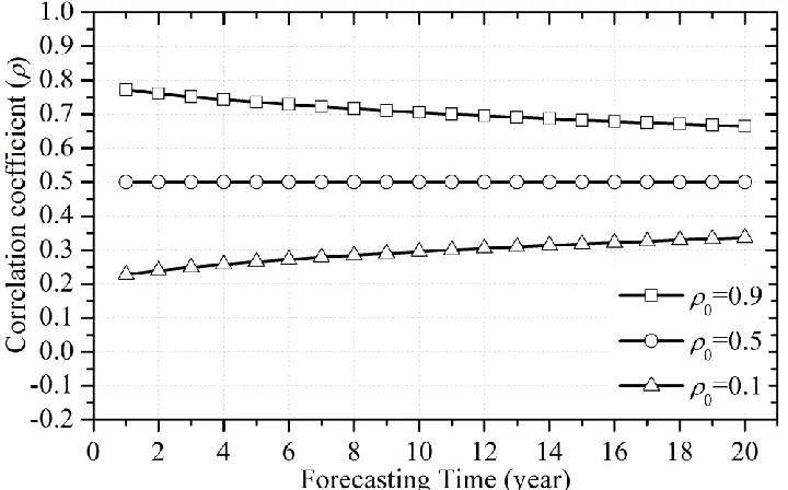
Figure 2.2 Correlation coefficient between linearized safety margins associated with different components for a degrading parallel system with five components ... 33

Figure 2.3 System failure probability for a degrading parallel system with five components 34 Figure 2.4. Correlation matrix of the safety margins associated with the eleven transmission towers in the tower-line system ... 34

Figure 2.5 Sensitivity of Pfsys and Pf1,3 to R (mR/mW = 1.25, vR = 0.12 and vW = 0.05) ... 35

Figure 2.6 Sensitivity of Pfsys to mR/mW, vR and vW (R= 0.2) ... 35

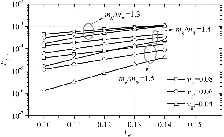
Figure 2.7 Sensitivity of Pf1,3 to mR/mW, vR and vW (0 = 0.2) ... 36

Figure 3.1 Illustration of the equivalent component approach for a series system with m components ... 55

Figure 3.2 Schematic illustration of effects of the combining sequence ... 55

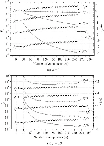
Figure 3.3 Accuracy of IECA for series systems with equicorrelated components ... 56

Figure 3.4 Impact of  on the accuracy of IECA for series systems with 250 equicorrelated components ... 57

Figure 3.5 Comparison of EPM, SCM and IECA for series systems with 250 equicorrelated components and c= 6 ... 58

Figure 3.6 Accuracy of equivalent component approach for series systems with unequally correlated components using correlation structure given by Eq. (3.12) ... 59

Figure 3.7 Accuracy of equivalent component approach for unequally correlated components with the correlation structure given by Eq. (3.15) (min = 0 and max = 0.98) ... 59

Figure 3.8 Accuracy of adaptive combing process for series systems with 250 components correlated according to Eq. (3.15) with max=0.98 and min varying from 0 to 0.98 ... 60

Figure 3.9 Comparison of accuracy and efficiency of EPM, SCM and IECA for series system with c= 6 and the component correlation structure defined by Eq. (3.12) ... 61

Figure 3.10 Time-dependent system reliability of the corroding pipeline joint ... 62

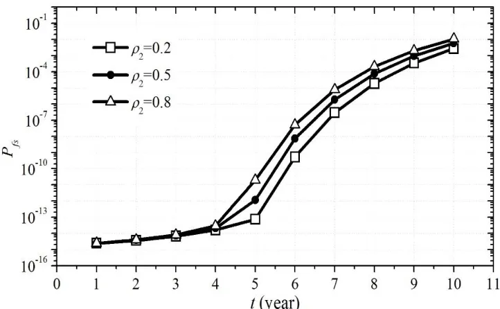
Figure 3.11 Sensitivity of the system reliability of the corroding pipeline joint to the correlation between the defect depth and length growth rates ... 62

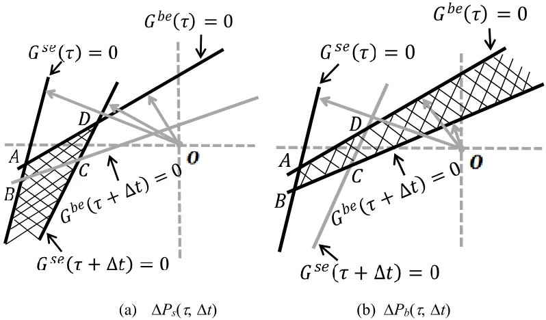
Figure 4.1Geometric descriptions of Ps(t) and Pb(t) ... 79

Figure 4.2 Probabilities of burst and small leak for examples 1, 2 and 3 based on the linear growth model for defect depth ... 82

Figure 4.3 Probabilities of burst and small leak for examples 1, 2 and 3 based on the nonlinear growth model for defect depth ... 85

Figure 4.4 Probabilities of burst and small leak for examples 1, 2 and 3 based on the homogeneous gamma process-based growth model for defect depth ... 88

Figure 5.1 Geometry descriptions of Ps(t)... 107

Figure 5.2 Failure probabilties of four pipeline examples considering a single corrosion defect and linear depth growth model ... 109

Figure 5.3. Failure probabilties of four pipeline examples considering ten corrosion defects and linear depth growth model ... 111

(10)

ix

(11)

x

List of Appendices

(12)

xi

List of Symbols

a, b = parameters of the gamma process

i,1 i,2 = the i-th elements of the unit normal vector for 1 and 2, respectively

𝛼_𝑖𝑠𝑒(𝑡)  the i-th element of se₍_t₎_

   unit vector normal to gU(u*)

j = unit normal vector associated with j

𝜶₁₂𝑒 = the n-dimensional unit normal vector associated with 𝑔₁₂𝑒 (𝒖) 𝜶′_(𝑗)_{ } _ __m_{-dimensional unit normal vector associated with}_𝒗∗_(𝑗) be₍_t₎ _{= equivalent unit normal vector associated with}_Gbe₍_t₎

se₍_t₎ _{= equivalent unit normal vector associated with}_Gse₍_t₎

 = reliability index

j = reliability index associated with the j-th limit state function

c = component reliability index value

be₍_t₎ _{= reliability index associated with}_Gbe₍_t₎

𝛽_•𝑒 = equivalent reliability index for equivalent component 𝐶_•𝑒

se₍_t₎ _{= reliability index associated with}_Gse₍_t₎

𝛽_𝑗𝑏(𝑡)   reliability index associated with Prob[𝑔_𝑗𝑏(𝑡) ≤ 0]

𝛽_𝑗𝑠(𝑡)   reliability index associated with Prob[𝑔_𝑗𝑠(𝑡) ≤ 0]

s₍_t₎ _{= reliability index vector of}_𝛽

𝑗𝑠(𝑡) (j=1, 2, …, m)    reliability index vector

C = present-value cost of excavation and repairing joints

C0 = mobilization cost

Ca,t = annual budget in terms of the present value allocated for corrosion repair at time t

Cm = the m-th component of a series system Cs = cost of repairing a single joint

Cr,t = present-value cost of repairs conducted at time t 𝐶_•𝑒 = equivalent compoment

COV = coefficient of variation

d = corrosion defect depth

d0 = initial corrosion defect depth d0j = initial depth of the j-th defect

dj(t) = depth of the j-th corrosion defect at a given time t

dgj(t) = homogeneous gamma process at the j-th defect at a given time t

dgj(t) = gamma-distributed increment of the defect depth within t d0j = initial depth of the j-th corrosion defect

D = actual outside pipe diameter

ep = error associated with estimated system failure probability EPM = Equivalent plane method

(•) = gamma function

fU(u) = joint standard normal probability density function of U fX(x) = the joint probability density function of X

(13)

xii

F0 = ratio of Zi,k relative to Xi,k 𝐹(•|•,•)  =gamma distribution

FR(•,•,…,•) = joint probability distribution of Rj FRj(•) = cumulative distribution function of Rj FX(•,•,…,•) = joint probability distribution of X

FXj(•) = cumulative distribution function of Xj(t) FWj(•) = cumulative distribution function of Wj FORM = First order reliability method

FPR = failure pressure ratio

𝑔₁₂𝑒 (𝒖) = equivalent linearized safety margin for C1 and C2 in terms of

u

gd = depth growth rate

gdj = depth growth rate of the j-th corrosion defect gl = length growth rate

glj = length growth rate of the j-th corrosion defect g(•) = limit state function

gj(•) = the j-th limit state function

gj(t) = the j-th limit state function at a given time t

𝑔_𝑗𝑏(𝑡) = limit state function for plastic collapse of the remaining ligament at the j-th defect at time t

𝑔_𝑗𝑠(𝑡) = limit state function, 𝑔_𝑗𝑠(𝑡), for the j-th defect penetrating the pipe wall at a given time t

gU(•) = limit state function in standard normal space U

gj,U(•) = the j-th limit state function in terms of random variable vector U

gj,Uj(•) = the j-th limit state function in terms of random variable vector

Uj

gZ(•) = limit state function in the correlated normal space Z

gj,Z(•) = the j-th limit state function in the correlated normal space Z gb₍_t₎ _{= limit state function for plastic collapse of the remaining}

ligament at one single defect at time t

gs₍_t₎ _{= limit state function for plastic collapse of the remaining} ligament at one single defect at time t

G(u) = mapping of g(x) in the standard normal (i.e. U) space

Gj(u) = mapping of gj(x) in the standard normal (i.e. U) space Gb₍_t₎ _{= mapping of}_gb₍_t_{) in the standard normal space}

Gs₍_t₎ _{= mapping of}_gs₍_t_{) in the standard normal space} 𝐺_𝑗𝑏(𝑡) = mapping of 𝑔_𝑗𝑏(𝑡) in the standard normal space

𝐺_𝑗𝑠(𝑡) = mapping of 𝑔_𝑗𝑠(𝑡) in the standard normal space

Gbe₍_t₎ _{= linearized equivalent limit state function at time}_t_representing the plastic collapse

Gse₍_t₎ _{= linearized equivalent limit state function at time}_t_representing the wall thickness penetration

GA = Genetic algorithm

hU(•) = IS density function in the standard normal space

(14)

xiii

ℎ_𝑼𝑠(𝒖; 𝜏, ∆𝑡) = weighted average of the IS density functions for Ps,j(t) I(•) = failure indicator function

𝐼_{(𝜏,∆𝑡)}𝑠 (•) = index functions associated with Ps(t) 𝐼_{(𝜏,∆𝑡)}𝑏 (•) = index functions associated with Pb(t)

Ir(nr,t) = an indicator function that equals unity for nr,t> 0 and zero for nr,t= 0

IECA = Improved equivalent component approach ILI = In-line inspection

IS = Important sampling

kj = parameters of the power-law growth model for the j-th defect l = corrosion defect length

l0 = initial depth of corrosion defect

l0j = initial length of the j-th corrosion defect

lj(t) = length of the j-th corrosion defect at a given time t

L, L(j) = lower-triangular matrix of Cholesky decomposition of RZZ,

RZZ(j)

LY = lower-triangular matrix obtained from Cholesky

decomposition of R

Lj,j, Lcj,j and Lcj,cj = submatrices of dimensions of nj × nj, (n-nj)× nj, and (n-nj)× (n-nj) of L(j), respectively

m = number of limit state functions, components or defects

mp = number of repaired pipe joints mR = mean value of FRj(•)

mW = mean value of FWj(•)

M = Folias factor

Mj = Folias factor at the j-th defect MC = Monte Carlo simulation MFL = magnetic flux leakage

MOP = Maximum operating pressure

n = number of random variable in the system

nj = number of random variables only involving gj(•)

 np = number of inspected pipe joints

nr,t = number of joints repaired at time t N = total number of IS trials

 = correlation coefficient value between two linearized safety margin

0 1 2 R = specified correlation coefficient value between random variables

minmax = pre-determined lower and upper bound values of correlation matrix

w(•) = correlation coefficient between Wj and Wk

Zi,k = correlation coefficient between Zi and Zk

Xi,k = correlation coefficient between Xi and Xk

jk = correlation coefficient between the linearized safety margins of the j-th and k-th components

(15)

xiv

pj = internal pressure at the j-th defect pb = burst capacity

pbj(t) = burst capacity at at the j-th defect at a given time t P0 = nominal maximum operating pressure

P1 P2 = allowable annual probabilities of maximum small leak and burst, respectively

Pb(t) Ps(t) = cumulative probabilities of burst and small leak of a pipeline joint,respectively, at a given time t

Pb,q(t) Ps,q(t) = the cumulative probabilities of burst and small leak , respectively, of the q-th joint up to t

PbaPsa = maximum value of Pba,q(t) and Pla,q(t) (t = 1, 2, …, T; q = 1, 2, …, np), respectively

Pba,q(t) Psa,q(t) = conditioned annual failure probabilities of burst and small small leak of the q-th joint, respectively, at a given time t Pf = system failure probability

Pf,q(t) = cumulative failure probability of the q-th joint Pf12 = series system failure probability of two components Pf1,3 = probability of simultaneous collapse of towers 1 and 3

Pfs = estimated failure probability of a series system Pfse = exact system failure probability

Pfsys = probability of collapse of at least one tower

Ps,q(t) Pb,q(t) = cumulative probabilities of small leak and burst, respectively up to t

Ps₍_t₎ _{= cumulative probability of any of defects penetrating the} pipe wall within [0, t]

rj = value of random variable Rj

rsb₍_₎ _{= correlation coefficient between}_Gse₍__{) and}_Gbe₍__). Rj = ultimate capacity of the j-th tower

R = correlation matrix of the linearized safety margins

Rs₍_t₎ _{= correlation matrix of the linearized safety margins associated} with 𝑔_𝑗𝑠(𝑡) (𝑗 = 1, 2, … , 𝑚) in standard normal space

Rsb₍__t₎ _{= correlation matrix of three linearized equivalent limit state} functions Gse₍_₊__t_),_Gse₍__{) and}_Gbe₍_₎

Rbs₍__t₎ _{= correlation matrix of three linearized equivalent limit state} functions Gbe₍_₊__t_),_Gbe₍__{) and}_Gse₍_₎

RZZ = correlation matrix of the elements in Z

RZZ(j) = correlation matrix of the elements in ZD(j)

RZj,j = correlation matrix of the elements in Zj

RZcj,cj = correlation matrix of the elements in Zcj

RZj,cj = correlation between the elements in Zj and Zcj SCM = sequential compounding method

SMTS = specified minimum tensile strength SMYS = specified minimum yield strength

t = forecasting time

tr,q = the time of repair for the q-th pipe joint

𝑡_𝑗𝑠 = time at which the j-th defect just penetrates the pipe wall

(16)

xv

T = inspection time horizon

u = the mean of the depth increment within one year

u = value of the vector U

ui = the i-th element of the vector u

ucj = value of the vector Ucj

uj = value of the vector Uj

u* = design point vector in the standard normal space

𝒖_𝑐𝑗∗ = vector of (n-nj) design point values that are not in uj* 𝒖_𝑖′ = i-th random sample generated from hU(u)

u*(j) = design point involving the whole system associated with j 𝒖_𝐷∗(𝑗) = vector of re-ordered elements of u*(j)

𝒖_𝑗∗ = design point value of Uj

uc*₍_₎ _{= design point associated with}_Gb₍_₎₌₀

ul*₍_₎ _{= design point associated with}_Gs₍_₎₌₀

ub*₍__,__t₎₎ _{= design point associated with}__P

b(t)

us*₍__,__t₎₎ _{= design point associated with}__P

s(t) 𝒖_𝑗𝑏∗(𝜏, ∆𝑡) = design points associated with Pb,j(t) 𝒖_𝑗𝑠∗(𝜏, ∆𝑡) = design points associated with Ps,j(t) Ui = the i-th element of the vector U

U =random variable vector in the standard normal space

UD(j) = a collection of Uj and Ucj, i.e., [UjT, UcjT]T

Uj = vector of nj independent standard normal variates involving gj(•) itself

Ucj = vector of (n-nj) random variables that are not in Uj UT = ultrasonic technology

v = coefficient of variation

vr = discount rate of the maintenance cost vW = coefficient of variation of FWj(•) vR = coefficient of variation of FRj(•)

𝒗∗_(𝑗) ₌_m_{-dimensional design point associated with}_𝒚∗_(𝑗)_{in the}

standard normal space

V = m-dimensional vector in the independent standard normal space

wj = weighting factor assigned to the IS density function associated with the j-th component

wtj = wall thickness random variable at the j-th defect wtn = nominal value of wall thickness

𝑤_𝑗𝑏(𝜏, 𝑡) = weighting factor for ℎ_𝑼𝑏(𝒖; 𝜏, ∆𝑡)

𝑤_𝑗𝑠(𝜏, ∆𝑡) = weighting factors for ℎ_𝑼𝑠(𝒖; 𝜏, ∆𝑡)

Wj, Wk = wind speed at the the j-th and the k-thtower, respectively xcj = value of Xcj

xj(t) = value of Xj(t)

x = value of the vector X xj = value of the vector Xj

(17)

xvi

𝒙_𝐷∗(𝑗) = design point in the XD(j) space

xj(uj) = function xj is defined in terms of uj

x(z) = function x defined in terms of z

Xcj = random variable of the critical threshold associated with the j-th component

Xi = the i-th element of the vector X

Xj(t) = random variable vector of the cumulative degradation within the interval [0, t] of the j-th component

X = random variable vector in the original space

Xcj = vector of (n-nj) random variables that are not in Xj

XD(j) = a collection of Xj and Xcj, i.e., [XjT, XcjT]T

Xj = vector of nj random variables involving gj(•)

y*₍_j₎ ₌_m_{-dimensional design point associated with the}_j_-th component in the correlated normal space

𝒚_𝐷∗_(𝑗) _{= re-ordered vector of design point}_y*₍_j₎

𝑦_𝑗∗ = one-dimensional design point associated with the j-th component

𝒚_𝑐𝑗∗ = the values of Yk (k= 1, 2, …, m; 𝑘 ≠ 𝑗)at the design point y*(j) yj = value of a standard normal variate Yj

Yj = the j-th element of the vector Y

Y =an m-dimensional correlated standard normal variates with the correlation matrix R

z = value of the vector Z

zj = value of normal variate Zj

𝒛_𝑗∗ = design point only involving the j-th limit state function in the correlated space

𝒛_𝑖𝑠 = the i-th m-dimensional random sample generated from h(•)

𝑧_𝑖𝑗𝑠 = the j-th (j = 1, 2, …, m) element of the vector 𝒛_𝑖𝑠

𝒛_𝑐𝑗∗ = (n-nj) elements of design point that are not in zj* in the correlated space

z*₍_j₎ _{= design point involving the whole system in the correlated} normal space associated with j

𝒛_𝐷∗_(𝑗) _{= design point in the space}_Z

D(j)

z(u) = function z defined in terms of u

Zj, Zk = the j-th, k-th element of the vector Z

Z =random variable vector in the correlated normal space

Zj = vector of nj random variables in the correlated normal space

Zcj = vector of (n-nj) random variables associated with Xcj in thecorrelated normal space

ZD(j) = a collection of Zj and Zcj, i.e., [ZjT, ZcjT]T

SC1, SC2 SC3 = solutions selected from the Pareto front with the constant budget constraint

SN1, SN2 = solutions selected from the Pareto front with no budget constraint

SV1, SV2 = solutions selected from the Pareto front with the variable budget constraint

(18)

xvii Constraint

   reduction factor

(•) = standard normal density function

2(•, •, •) = probability density function of the bivariate normal distribution

m(•,•) = m-dimensional normal probability density function 

(•) = standard normal cumulative distribution function

₍_•₎ _{= the inverse of the standard normal cumulative distribution}

function

m(•,•) = m-variate standard normal distribution function

2(β1, β2, 12) = bivariate cumulative normal function evaluated at [β1 β2]T wit correlation coefficient of 12

i, k = coefficients of variation of Xi and Xk, respectively

n-_nj = (n-nj)-dimensional vector of zeros

1(∙) = inverse normal transformation operator

   standard deviation of the depth increment within one year u = ultimate tensile strength

uj = ultimate tensile strength at the j-th defect

yj = yield strength at the j-th defect

𝜉_𝑗 = model error associated with burst capacity model at the j-th defect

jk = distance between the j-th and k-th tower sites

dj(t) lj(t) = growths of the depth and length of the j-th defect, respectively, by time t

Pb,j(t) = incremental probability of burst between and  + t for the j-th defect

Ps,j(t) = incremental probability of small leak between and  + t for the j-th defect

Ps(t) Pb(t) = incremental probabilities of small leak and burst, respectively, within a short time interval between  and + t.

t = incremental time interval ||•|| = norm of a vector

Ω(x) = failure domain with x being the value of X

Ω'(u) = failure domain with u being the value of U

b₍__,__t₎ _{= failure domain associated with}__P

b(t)

s₍__,__t₎ _{= failure domain associated with}__P

(19)

1 Introduction

1.1 Background

Onshore pipeline systems are generally recognized as the safest and most economical way to transport oil and gas in a long distance. Failures of pipelines do occur occasionally and are associated with severe consequences in terms of the human safety, property damage and environmental impact. Pipelines are required to be well maintained to ensure safe operation throughout the service life. However, pipeline operators are faced with limited financial resources for maintenance. To achieve a desirable solution between pipeline safety and economic viability, the optimal maintenance strategy for in-service pipelines should be explicitly investigated.

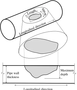
Metal loss corrosion is one major failure cause for onshore pipelines (EGIG 2015; Nessim et al. 2009). Corrosion caused 35% of failures on oil and gas transmission pipelines in Canada between 2010 and 2014 (CEPA 2015) and 32% of reportable incidents on gas transmission pipelines in the US between 2002 and 2013 (Lam and Zhou 2016). A typical corrosion defect is three-dimensional and characterized by its length (in the pipeline longitudinal direction), width (in the circumferential direction) and maximum depth (in the through-pipe wall thickness direction). A representative corrosion defect is showed schematically in Fig. 1.1. Corrosion defects grow actively in length and depth over time. In-Line Inspections (ILI), relying on the Magnetic Flux Leakage (MFL) or ultrasonic technology (UT), are now being commonly employed by pipeline operators to detect, locate and size corrosion defects on the surfaces of pipelines at a regular interval varying from a few to ten years (Kariyawasam and Peterson 2010).

(20)

Industry practice is to mitigate corrosion defects on a joint-by-joint basis as opposed to a defect-by-defect basis (Zhang and Zhou 2014); that is, mitigating a critical corrosion defect requires the excavation of the entire pipe joint containing the defect and repairing (or replacing) the joint. Condition assessment of corroding joints based on the defects reported by ILI tool is a critical part of developing excavation and repairing schedules. Integrity engineer carries out the deterministic or probabilistic defect assessment (Kariyawasam and Huyse 2012; Zhou et al. 2016). The deterministic assessment requires evaluating the Failure Pressure Ratio (FPR) between the nominal burst pressure capacity at the defect and the Maximum Operating Pressure (MOP) of the pipeline (Kariyawasam and Huang 2014). Any defect with FPR less than the pre-defined threshold (e.g., 1.1 or 1.25) is considered critical and the joint containing such a defect is excavated and repaired. The probabilistic defect assessment involves calculating the burst failure probability at the defect, and the one with probability of burst exceeding the pre-defined threshold (e.g. 10-3_{) is deemed} critical. The latter is increasingly employed in industry practice for quantifying the pipeline safety (Kariyawasam and Peterson 2010; Huyse and Brown 2012), chiefly for the advantages of managing various relevant uncertainties such as model error, wall thickness, and pressure et al. However, a single pipeline joint, typically with length of 10 - 20 m long (Al-Amin and Zhou 2014), may contain multiple active corrosion defects. The joint with a single defect is less critical than the one containing more defects with the same size. The joint should be considered as a series system in the reliability assessment. The correlation between the defect sizes, operating pressure and pipe properties (e.g. pipe wall thickness and yield strength) at different defects can result in correlated failures at different defects. Such correlations must be dealt with. Small leak and burst are mutually competing against each other. The occurrence of one failure mode, either small or burst, would eliminate the occurrence probability of the other.

(21)

introduced in the literature (Teixeira et al. 2008; Sahraoui et al. 2013; Zhang and Zhou 2014; Miran et al. 2016). However, those methods either ignore the competing characteristics of small leak and burst failures, or fail to consider multiple correlated corrosion defects as a series system. The application of the FORM to the system reliability analyses relies on the design points to calculate the correlation coefficients between the failures at different defects and the multi-normal integral to evaluate the system reliability. The design point is obtained from the constrained optimization while the multi-normal integral is a function of reliability index at different defects and associated correlation coefficients. With an increased number of defects, the dimension of both optimization and multi-normal integral increases (Kang and Song 2010; Roscoe et al. 2015). It follows that the efficiency of the FORM may be therefore hampered.

(22)

1.2 Objective and Research Significance

The research described in this thesis is financially supported by Natural Sciences and Engineering Research Council (NSERC) of Canada and TransCanada Ltd. The objective of this research is summarized as follows:

1) Development of efficient methods to obtain the design points for limit state functions in the system reliability application of the FORM;

2) Development of efficient multi-normal integral methods within the FORM for large series systems with significant number of correlated components;

3) Development of the FORM and important sampling (IS) based methodology for assessing small leak and burst system failure probabilities incorporating the competing characteristics;

4) Development of the optimum cost-effective maintenance strategy for corroding pipeline systems, with the consideration of the conflicting safety and cost objectives. It is expected that the contribution in this thesis will be beneficial for the reliability assessment of large systems in various other disciplines in addition to pipeline systems. Moreover, it will also facilitate the integrity maintenance management of in-service corroding pipeline systems.

1.3 Scope of Study

(23)

Chapter 3 presents an improved equivalent component approach to evaluate the system reliability of series systems by providing an analytical expression to evaluate the unit normal vector, in the context of the FORM, associated with the equivalent component. It is also proposed that the two components with the highest correlation coefficient be combined at each combining step. The accuracy and efficiency of the adaptive equivalent component approach are demonstrated to be excellent for series systems with equi-correlated and unequally equi-correlated components through various examples.

Chapter 4 introduces a methodology that employs the FORM to evaluate the time-dependent system reliability of a joint of a pressurized pipeline containing multiple active corrosion defects. The methodology considers small leak and burst failure modes of the pipeline joint, and accounts for the correlations among limit state functions at different corrosion defects. The methodology involves first constructing two linearized equivalent limit state functions for the pipe joint in the standard normal space and then evaluating the probabilities of small leak and burst of the joint incrementally over time based on the equivalent limit state functions.

In Chapter 5, an IS technique-based method is introduced to evaluate the time-dependent system reliability of corroding pipeline joints containing multiple active corrosion defects by considering two competing failure modes, i.e., small leak and burst. The IS density functions in the standard normal space for incremental probabilities of small leak and burst of the pipeline joint over a short time interval are established as the weighted averages of the IS density functions for small leak and burst, respectively, at individual corrosion defects. The IS density functions for incremental probabilities of small leak and burst at individual defects are centered at the design points associated with corresponding failure domains.

(24)

specified initial population is employed to improve the robustness of obtaining a complete Pareto front.

It is assumed throughout this thesis that sizes of corrosion defects are monotonically increasing with time. Both stochastic process- and random variable-based defect growths are considered in the work reported in the thesis. Once repaired, a corroding pipe joint is restored to the pristine condition. All pipelines are accessible to ILI. The reliability analysis is carried out based on the corrosion defect information provided by a recently-run ILI. Since a future ILI will provide the updated information for corrosion defects, the time-dependent reliability analysis is generally carried out up to the time of the next ILI.

1.4 Thesis Format

This thesis is prepared in an Integrated-Article Format as specified by the School of Graduate and Postdoctoral Studies at Western University, London, Ontario, Canada. In total, seven chapters are included in the thesis. Chapter 1 is the introduction of the whole thesis, describing the research background, objectives and scope. Chapter 2 through Chapter 6 are the main body of the thesis, where each chapter acts as a stand-alone manuscript that is the key part of the published papers and submitted manuscripts. In the last chapter, conclusions of the thesis and recommendations for the future work are summarized.

1.5 References

Al-Amin, M., and Zhou, W. (2014). Evaluating the system reliability of corroding pipelines based on inspection data. Structure and Infrastructure Engineering, 10(9), 1161-1175.

Canadian Energy Pipeline Association (CEPA). (2015). Committed to safety, committed to Canadians. 2015 pipeline performance report. Calgary, Alberta: Canadian Energy Pipeline Association.

(25)

Huyse, L., and Brown, K. A. (2012). Why reliability-based approaches need more realistic corrosion growth modeling. 9th International Pipeline Conference (IPC2012), ASME, IPC2012-90319, Calgary, Alberta, Canada

Kang, W. H., and Song, J. (2010). Evaluation of multivariate normal integrals for general systems by sequential compounding. Structural Safety, 32(1), 35-41.

Kariyawasam, S., and Huang, T. (2014). How safe failure pressure ratios are related to% SMYS. In 2014 10th International Pipeline Conference (pp. V002T06A019-V002T06A019). American Society of Mechanical Engineers.

Kariyawasam, S., and Huyse, L. (2012). Providing Safety: Using Probabilistic or Deterministic Methods. In 2012 9th International Pipeline Conference (pp. 725-734). American Society of Mechanical Engineers.

Kariyawasam, S., and Peterson, W. (2010). Effective improvements to reliability based corrosion management. 8th International Pipeline Conference (IPC2010), ASME, IPC2010-31425, Calgary, Alberta, Canada

Lam, C., and Zhou, W. (2016). Statistical analyses of incidents on onshore gas transmission pipelines based on PHMSA database. International Journal of Pressure Vessels and Piping, 145, 29-40.

Miran, S. A., Huang, Q., and Castaneda, H. (2016). Time-dependent reliability analyses of corroded buried pipelines considering external defects. Journal of Infrastructure Systems, 22(3), 04016019.

Nessim, M., Zhou, W., Zhou, J., and Rothwell, B. (2009). Target reliability levels for design and assessment of onshore natural gas pipelines. Journal of Pressure Vessel Technology, 131(6), 061701.

(26)

Sahraoui, Y., Khelif, R. and Chateauneuf, A. (2013). Maintenance planning under imperfect inspections of corroded pipelines. International Journal of Pressure Vessels and Piping, 104, 76-82.

Teixeira, A. P., Soares, C. G., Netto, T. A. and Estefen, S. F. (2008). Reliability of pipelines with corrosion defects. International Journal of Pressure Vessels and Piping, 85(4), 228-237.

Zhang, S. and Zhou, W. (2014). Cost-based optimal maintenance decisions for corroding natural gas pipelines based on stochastic degradation models. Engineering Structures, 74, 74-85.

Zhang, S. and Zhou, W. (2014). An Efficient Methodology for the Reliability Analyses of Corroding Pipelines. Journal of Pressure Vessel Technology, 136(4), 041701.

Zhou, W. (2010). System reliability of corroding pipelines. International Journal of Pressure Vessels and Piping, 87(10), 587-595.

Zhou, W., Gong, C., and Kariyawasam, S. (2016). Failure Pressure Ratios and Implied Reliability Levels for Corrosion Anomalies on Gas Transmission Pipelines. In 2016 11th International Pipeline Conference (pp. V001T03A017-V001T03A017). American Society of Mechanical Engineers.

(27)

Figure 1.1Schematic illustration of the geometry of a typical corrosion defect

Longitudinal direction

Maximum depth Pipe wall

(28)

2 New Perspective on the Application of the First-order

Reliability Method for Estimating System Reliability

2.1 Introduction

The reliability of a system governed by a single limit state function can be calculated

efficiently using the well-known first-order reliability method (FORM) (Hasofer and Lind

1974; Veneziano 1974; Rackwitz and Fiessler 1978). The calculation involves

transforming the random variables involved in the limit state function into the standard

normal space and evaluating the reliability index, which equals the minimum distance from

the origin to the limit state surface in the standard normal space. The application of the

FORM also provides a vector of sensitivity factors at the solution point (i.e., design point)

on the limit state surface in the standard normal space (Madsen et al. 2006). Moreover, the

FORM assumes that the limit state function is approximated by a linearized safety margin,

resulting in the limit state surface being approximated by a tangential hyperplane passing

the design point.

If the performance of a system is governed by many limit state functions, the system

reliability analyses must consider all the limit state functions and correlations between the

corresponding safety margins (Straub and Faber 2005; Der Kiureghian 2005; Madsen et al.

2006; Kang et al. 2012). To take the correlation into account, the application of the FORM

to each limit state function is carried out by mapping the random variables in the entire

system into the normal space, and the correlation coefficients between the linearized safety

margins for any two limit state functions are calculated using the vectors of sensitivity

factors at the respective design points (Melchers 1999; Madsen et al. 2006; Ang and Tang

2007). In such a case, the number of random variables involved in the FORM analyses for

each limit state function in the transformed normal space may be much greater than that is

required for the limit state function in the original space. This increase in the dimensions

of the analyses space reduces the computational efficiency and robustness of the FORM.

The above-observed deficiency in using the FORM to calculate the system reliability is

relevant to many practical problems. For example, a corroding pipeline may contain many

(29)

corrosion defects are correlated if, for example, the sizes of different defects are correlated.

This correlation increases the number of random variables involved in the FORM analyses

for each individual defect in the standard normal space if the system reliability aspect is

considered. Another example is a tower-line system with several transmission towers that

are subjected to spatially correlated wind loads (or ice loads or earthquake loads) (Hong et

al. 2006, Zhang and Li 2007; Chen and Booth 2011). As a first order approximation,

assume that the wind load on each tower can be characterized by the time averaged mean

wind speed at the tower site and that the tower capacity can be presented by the nonlinear

static pushover curve (Mara and Hong 2013). To evaluate the system reliability of the

tower-line systems, the wind load in the FORM analyses for each individual tower needs

to be expressed as a combination of standard independent normal variates due to the spatial

correlation of the wind loads. This increase in the number of random variables reduces the

computational efficiency and robustness of using the FORM to calculate the failure

probability of each tower.

In short, the use of the FORM to calculate the reliability of engineering systems could be

inefficient if there are many limit state functions involved in the system and each limit state

function is a function of only a few random variables in the original space but a large

number of random variables for the system in the transformed normal space. A new

efficient procedure for calculating the correlation coefficients between the safety margins

associated with different limit state functions in the system reliability analyses is proposed

in this chapter. The basic steps of the procedure are to 1) apply the FORM to each limit

state function by considering only the random variables involved in the limit state function

(as opposed to the entire system); 2) identify the design point for each limit state function

by considering all random variables for the system based on the results obtained in Step 1);

and 3) find the correlation coefficients among the linearized safety margins. Steps 1) - 3)

involve the application of a new theorem put forward in this chapter. In the following

sections, the basic concept of the FORM is summarized, and the new theorem is presented.

The application of the procedure to several practical system reliability analyses problems

(30)

2.2 Basics of the First-order Reliability Method

2.2.1 Analyses for a Single Limit State Function

The basic concept of the FORM is explained in several well-known references, including

Melchers (1999), Madsen et al. (2006), and Ang and Tang (2007). It is used to evaluate

approximately the failure probability, Pf, represented by the following multidimensional

integral

𝑃_𝑓 = ∫_{𝑔(𝒙)≤0}𝑓_𝑿(𝒙)𝑑𝒙 (2.1)

where x denotes values of a vector of random variables X = [X1, X2, …, Xn]T; g(x) is the limit state function with g(x) > 0 and g(x) < 0 defining the safe and failure domains, respectively; g(x) = 0 is known as the limit state surface, and fX(x) is the joint probability

density function of X. The FORM is carried out by transforming X into Z = [Z1, Z2, …, Zn]T, and Z to U = [U1, U2, …, Un]T, where Zi (i = 1,…, n) are correlated normal variates with zero means and unity variances, and Ui are independent and standard normal variates.

The reliability index  is then given by

𝛽 = min

𝑔𝑍(𝒛)=0

√𝒛T_𝑹 𝒛𝒛

−1_𝒛 _(2.2)

or,

𝛽 = min

𝑔𝑈(𝒖)=0

√𝒖T_𝒖 _(2.3)

where z denotes the value of Z; u denotes the value of U; RZZ is the correlation matrix of

Z, gZ(z) = g(x(z)) is the limit state function in terms of z; x(z) denotes that x is a function of z; gU(u) = g(x(z(u))) is the limit state function in terms of u, and z(u) denotes that z is a function of x. The equivalence of Eqs. (2.2) and (2.3) is well established in the context of the first-order second-moment reliability method (Veneziano 1974; Hasofer and Lind

1974). The meaning of Eq. (2.2) in the context of the FORM is explained by Low and

Tang (2007); that is,  is the axis ratio of a multi-normal dispersion ellipsoid that just

(31)

The spreadsheet-based implementation of Eq. (2.2) for simple practical applications is also

described in Low and Tang (2007).

The transformation from X to Z for dependent or correlated Xi using the Nataf transformation is extensively discussed in Der Kiureghian and Liu (1986) and Der

Kiureghian (2005). The use of the (unidimensional) inverse normal distribution and Nataf

transformation provides a one-to-one mapping from Xi to Zi. Let Zi,k (i, k = 1, 2, …, n; i ≠

k) denote the correlation coefficient between Zi and Zk, and Xi,k denote the correlation

coefficient between Xi and Xk. Then Zi,k can be evaluated from Xi,k as (Der Kiureghian and Liu 1986)

𝜌_{𝑍𝑖,𝑘} = 𝐹₀ ∙ 𝜌_{𝑋𝑖,𝑘} (2.4)

where F0 ( ≥ 1) is in general a function of Xi,k and parameters of the marginal distributions of Xi and Xk, and can be estimated using the empirical equations for various marginal

distributions given in Der Kiureghian and Liu (1986). The empirical equations that are

employed for the numerical examples considered in this chapter are summarized in Table

2.1. The transformation from Z to U can be carried out by employing U = L-1Z, where L

is the lower-triangular matrix obtained from the Cholesky decomposition of RZZ (Der

Kiureghian 2005).

The failure probability, Pf, is then approximated by

Pf = (-) (2.5)

(32)

2.2.2 Observed Deficiency for System Reliability Analyses with

Multiple Limit State Functions

Consider a system reliability problem that is defined by m limit state functions, gj(xj) (j = 1, 2, …, m), where xj is the value of Xj representing a vector of nj random variables that need to be considered for gj(xj). Let X denote the union of all Xj, representing a vector of n random variables that needs to be considered for the system, whereby n can be much

greater than nj.

If the reliability analyses for a single limit state gj(xj) is of interest, the FORM procedure is the same as that shown in the previous section (see Eqs. (2.2) and (2.3)). However, since

the safety margins could be correlated and their correlations must be evaluated for

estimating the system reliability (Madsen et al. 2006; Der Kiureghian 2005), the most direct

application of the FORM in the context of the system reliability is to first transform X into

Z and/or U, where the symbols Z and U are already defined in the previous section. In the transformed spaces, the reliability index j for the j-th limit state function mentioned in the previous paragraph is then given by

𝛽_𝑗 = min

𝑔𝑗,𝑍(𝒛)=0

√𝒛T_𝑹 𝒛𝒛

−1_𝒛 _(2.6)

or,

𝛽_𝑗 = min

𝑔𝑗,𝑈(𝒖)=0

√𝒖T_𝒖 _(2.7)

where gj,Z(z) = gj(xj(z)) is the limit state function in terms of z, and gj,U(u) = gj(xj(z(u))) is the limit state function in terms of u. The design point corresponding to j is denoted by

u*(j). Both Eqs. (2.6) and (2.7) involve n-dimensional vectors of random variables in the transformed spaces, which decreases the computational efficiency and robustness of using

the FORM to evaluate j, as compared to the case where the FORM is applied to gj(xj) without considering the system reliability aspect. The decrease in the efficiency can be

very significant, especially for n much greater than nj, because the number of calls to the

limit state function in the FORM is proportional to the number of random variables in the

(33)

Because the limit state surface gj,U(u) = 0 is approximated by a hyperplane defined by j –

jTu = 0, where j = u*(j)/j, the correlation coefficient between the safety margins at the

solution points for the j-th and k-th limit states, jk, equals jTk (Madsen et al. 2006). In particular, the failure probability of system, Pf, can be expressed as

𝑃𝑓 = 1 − ∫ ⋯ ∫

1

√(2𝜋)𝑚|𝚺|exp (− 1 2𝛉

T_𝑹−1_𝛉) 𝛽𝑚

−∞ 𝑑θ1⋯ 𝑑θ𝑚

𝛽1

−∞ (2.8a)

if the system is a series system, and

𝑃_𝑓 = ∫ ⋯ ∫ 1

√(2𝜋)𝑚_|𝚺|exp (−

1 2𝛉

T_𝑹−1_𝛉) ∞

𝛽𝑚 𝑑θ1⋯ 𝑑θ𝑚

∞

𝛽1 (2.8b)

if the system is a parallel system, where R denotes the correlation matrix of standard normal variates with diagonal elements equal to one and off-diagonal elements defined by jk; and

 = [1, 2, …, m]T denotes an m-dimensional vector of standard normal variates with zero

mean and unity variance. Many approaches for evaluating the integrals in Eqs. (2.8a) and

(2.8b) have been proposed in the literature, for example, the Ditlevsen bounds (Ditlevsen

1979); equivalent component method (Gollwitzer and Rackwitz 1983; Estes and Frangopol

1998; Roscoe et al. 2015), sequential compounding method (Kang and Song 2010), and

quasi-Monte Carlo algorithms developed by Genz (1992, 1993), which have been

implemented in commonly used software packages such as Matlab and R (the

corresponding commands in Matlab and R are mvncdf(x, mu, sigma) and pmvnorm(upper

= c, corr = R)), respectively. Moreover, Eqs. (2.8a) and (2.8b) can be further simplified

for particular forms of the correlation matrix (Genz 1992, 1993). Discussions on evaluating

Pf for systems involving both series and parallel subsystems can be found in Der

Kiureghian (2005), Madsen et al. (2006) and Kang et al. (2012).

2.3 Efficient Procedure to Carry Out System Reliability

Analyses

(34)

Theorem: Consider that the vector X of all the n random variables that need to be considered for a system can be divided into two sub-vectors of random variables Xj and Xcj,

where Xj is a vector of nj random variables that need to be considered for gj(xj), and Xcj is

a vector of (n-nj) random variables that are not in Xj. Within the context of the Nataf transformation and FORM, the design point in the n-dimensional standard normal space is

given by *

j j

n n

 

 

  u

and the reliability index j, is given by,

𝛽𝑗 = min

𝑔_{𝑗,𝑈𝑗}(𝒖𝒋)=0

√𝒖𝑗T𝒖𝑗 (2.9)

where n-_nj denotes an (n-nj)-dimensional vector of zeros; uj* is the design point obtained by solving Eq. (2.9); gj,_Uj(uj) = gj(xj(uj))) is the limit state function in terms of uj; uj denotes the value of Uj that represents a vector of nj independent standard normal variates transformed from Xj; and xj(uj) emphasizes that xj is a function of uj.

To show that the above holds, consider XD(j) = [XjT, XcjT]T. Note that XD(j) is not necessarily equal to X because the orders of the random variables in XD(j) and in X could differ. By applying the (unidimensional) inverse normal transformation to each of the random variables in XD(j), denoted as 1(XD(j)) (i.e., 1(∙) represents an element to element inverse normal transformation operator) a vector of n zero mean and unity variance normal variates, ZD(j) = 1(XD(j)), is obtained. Similar to XD(j), ZD(j) is divided in two sub-vectors,