Scholarship@Western
Scholarship@Western
Electronic Thesis and Dissertation Repository
9-11-2015 12:00 AM
Structure-Function Relationship of the Brain: A comparison
Structure-Function Relationship of the Brain: A comparison
between the 2D Classical Ising model and the Generalized Ising
between the 2D Classical Ising model and the Generalized Ising
model
model
Pubuditha M. Abeyasinghe The University of Western Ontario
Supervisor Dr. Andrea Soddu
The University of Western Ontario Graduate Program in Physics
A thesis submitted in partial fulfillment of the requirements for the degree in Master of Science © Pubuditha M. Abeyasinghe 2015
Follow this and additional works at: https://ir.lib.uwo.ca/etd
Part of the Computational Neuroscience Commons
Recommended Citation Recommended Citation
Abeyasinghe, Pubuditha M., "Structure-Function Relationship of the Brain: A comparison between the 2D Classical Ising model and the Generalized Ising model" (2015). Electronic Thesis and Dissertation Repository. 3239.
https://ir.lib.uwo.ca/etd/3239
This Dissertation/Thesis is brought to you for free and open access by Scholarship@Western. It has been accepted for inclusion in Electronic Thesis and Dissertation Repository by an authorized administrator of
COMPARISON BETWEEN THE 2D CLASSICAL ISING MODEL AND
THE GENERALIZED ISING MODEL
(Thesis format: Monograph)
by
Pubuditha Abeyasinghe
Graduate Program in Physics
A thesis submitted in partial fulfillment
of the requirements for the degree of
Master of Science
The School of Graduate and Postdoctoral Studies
The University of Western Ontario
London, Ontario, Canada
c
There is evidence that the functional patterns of the brain observed at rest using fMRI are
sustained by a structural architecture of axonal fiber bundles. As neuroimaging techniques
advance with time, the relationship between structure and function has become the object of
many studies in neuroscience. As recently suggested, the well-defined connectivity structure
found in the brain can be used to understand the self organization of the brain at rest, as well as
to infer the functional connectivity patterns of the brain using different models. These models
include the Kuramoto model, which studies synchronization, and the two-dimensional classical
Ising model, which studies the global dynamics of the brain at the critical temperature. These
models have been successful in capturing the underlying properties of the brain. To extend this
understanding, our objective is to develop the generalized Ising model, following the lesson
from the two-dimensional Ising model, as the generalized Ising model could be simulated
using the anatomical structure of the brain. This model can then be used to study functional
information integration and segregation in the brain at rest. Thus, the primary research question
would be: can the generalized Ising model explain the functional behaviour of the resting brain
at the critical temperature? Preliminary analyses were carried out to determine the critical
temperature of the models and to compare the correlation distributions. Further analyses were
carried out using graph theory considering the brain as a network. By observing the results
obtained from our simulations, it can be inferred that there is a temperature that is different
from the critical temperature of the model at which the generalized Ising model shows a match
with the empirical functional connectivity. At that temperature, the generalized Ising model
could be used to study the global dynamics, as well as the local dynamics of the brain.
Keywords: Ising model, Structure and function of the brain, Graph Theory
To my family,
for their unconditional love and care...
To my adorable nephew,
for his priceless love and the biggest heart...
The preparation and compilation of this Dissertation would not have been possible if not for
the assistance and support given to me by my seniors, family and friends.
I would like to take this opportunity to extend my gratitude to my advisor, Prof. Andrea
Soddu for the assistance he rendered to me and for the amount of tolerance he demonstrated
when directing me in the correct path to make this dissertation a success. I must state that it was
a privilege to be guided by you. My extended gratitude goes towards my advisory committee
for spending their time to evaluate my work and to have all the meaningful discussions in order
to give me the opportunity to learn.
I also wish to extend my sincere thanks to Dr. Tushar K. Das for the support and for the
motivation he provided for my success from the beginning. Further, I thank all the members in
our group whom I met at some point in the past two years.
My heartfelt thanks are extended to all my friends who stood beside me during this journey
and who were supportive throughout.
Further, I thank my two brothers and sister for always being there with me whenever I need,
despite miles apart.
Finally, I thank my parents for being the biggest and the strongest pillers of my life. Even
though they are thousands of miles away, they managed to be with me the entire journey. I
would have performed less if it was not for their love and care. Special thanks goes to them,
for understanding my flaws, accepting me for who I am and for being closer to my heart always.
Contents
Abstract ii
Dedication iii
Acknowledgement iv
List of Figures viii
List of Tables xi
1 Introduction 1
1.1 Introduction . . . 1
1.2 Motivation & Objectives . . . 2
1.3 Thesis Outline . . . 3
2 Background & related work 4 2.1 Overview . . . 4
2.2 Neuronal Communication . . . 5
2.2.1 Functional Connectivity . . . 7
2.2.2 Structural Connectivity . . . 8
2.3 Brain Imaging . . . 9
2.3.1 Functional Magnetic Resonance Imaging (fMRI) . . . 9
2.3.2 Diffusion Tensor Imaging (DTI) . . . 12
2.4 Modelling the Brain . . . 14
Generalized Kuramoto Model . . . 16
2.4.2 Ising model . . . 17
Two dimensional (2D) Classical Ising Model . . . 17
Generalized Ising model . . . 21
2.4.3 Generalized Kuramoto Model versus Generalized Ising model . . . 23
2.5 Graph Theory . . . 24
3 Methodology 27 3.1 Overview . . . 27
3.2 Empirical Data from MRI . . . 27
3.2.1 Subjects . . . 27
3.2.2 Acquisition & Preprocessing . . . 28
Functional Data . . . 28
Structural Data . . . 28
3.2.3 Resting State Network (RSN) extraction . . . 29
3.3 Numerical Simulations . . . 29
3.3.1 Generalized Ising Model . . . 29
3.3.2 2D Classical Ising Model . . . 32
3.4 Comparison of data . . . 33
4 Results 35 4.1 Overview . . . 35
4.2 The Classical Ising model versus the Generalized Ising model . . . 35
5 Discussion and Conclusions 46 5.1 Future Directions . . . 51
Bibliography 52
.1 Appendix A: MATLAB code for simulations of the generalized Ising model . . 58
.2 Appendix B: Supplementary figures . . . 62
.3 Appendix C: Labels of 83 Parcellations of the Brain . . . 65
.4 Appendix D: Representation of the Resting State Networks . . . 68
Curriculum Vitae 69
2.1 Main components of a neuron [1] . . . 6
2.2 Main components of an MRI system. Image courtesy of the National Magnetic
Field Laboratory [2] . . . 10
2.3 BOLD time course of a patch of cortex from a brain at rest. . . 12
2.4 Lateral view of the white matter tracts in the brain, created by DTI. The
col-ors, red, blue and green represent the fibers along the x, y and z directions
respectively in the cartesian coordinates (DR Paula et al. in prep.) . . . 14
2.5 Representation of a two-dimensional lattice arrangement. Each lattice site has
a spin, either up or down. The nearest neighbours of the lattice site in green are
represented in red. . . 18
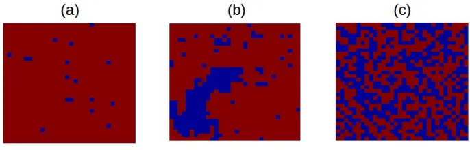
2.6 Representation of the equilibrium spin configuration for (a)T <Tc, (b)T = Tc
and (c)T > Tc for a two-dimensional lattice arrangement. Red color is for the
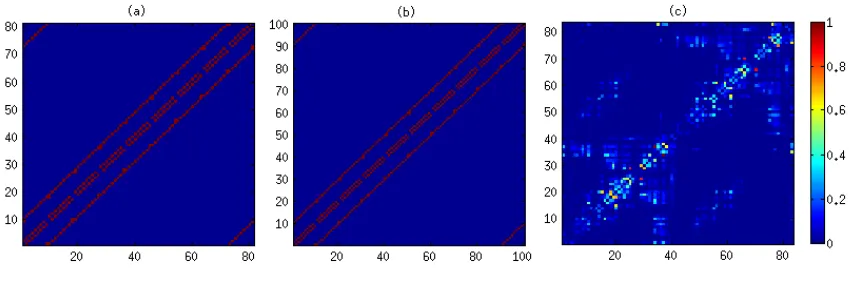
up spins (+1) and blue color is for the down spins (−1) [3]. . . 20 3.1 Connectivity matrices used for the simulations of the classical Ising model (a)
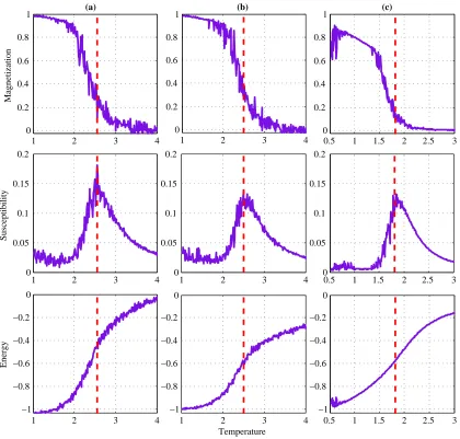
9×9 , (b) 10×10, and (c) the generalized Ising model. . . 32 4.1 Magnetization, susceptibility and Energy as a function of temperature for the
Classical Ising model with (a) 9× 9 and (b) 10× 10 lattice size, and (c) the Generalized Ising model. Red dashed line indicates theTc. . . 36
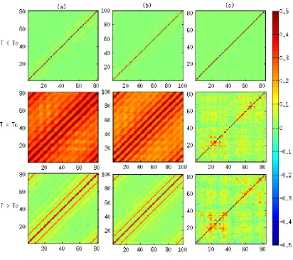
4.2 Correlation atT < T c,T = T c, andT > T cfor the classical Ising model with (a) 9×9 and (b) 10×10 lattice sizes, and (c) the generalized Ising model. . . . 37
lattice sizes and (c) the generalized Ising model as a function of temperature.
Red dashed line indicates the critical temperature for each model. . . 38
4.4 Simulated correlation matrices atT∗ for the classical Ising model with (a) 9×
9 and (b) 10×10 lattice sizes and (c) the generalized Ising model together with (d) the empirical correlation matrix. . . 39
4.5 Distribution of the correlation at T < Tc,T = Tc,T > Tc andT = T∗ for the
classical Ising model with (a) 9× 9 and (b) 10 × 10 lattice sizes, and (c) the generalized Ising model with the distribution of the correlation for empirical
data (EMP). The frequency in the y-axis is the normalized frequency. . . 40
4.6 Variation of the average degree as a function of the threshold. Top three
pan-els give the average degree with positive correlation for the (a) Classical Ising
model: 9 × 9, (b) Classical Ising model: 10 × 10 and (c) Generalized Ising model. The bottom three panels show the average degree for the negative
cor-relation for (d) Classical Ising model: 9×9, (e) Classical Ising model: 10×10 and (f) Generalized Ising model. . . 41
4.7 Graph theoretical properties as a function of temperature for the classical Ising
model with (a) 9×9 and (b) 10×10 lattice sizes, and (c) the generalized Ising model. The thick solid line represents threshold=0, the dashed line represents
threshold=0.07 and the thin solid line represents threshold=0.14. The black
lines represent the properties of the empirical data for the above thresholds.
The red and green vertical lines represent theTcandT∗respectively. . . 42
4.8 Connectivity graphs for the generalized Ising model for four temperatures,
along with the connectivity graph of the empirical network, thresholded at 0.07.
The color and the size of the nodes represent the degree. The darker the color
and larger the size, the higher the degree of each node in the network. . . 44
different temperatures, together with the empirical brain networks. Networks:
DMN=Default Mode Network, ECN l=External Control Network left, ECN r
=External Control Network right, Visua o=Visual Occipital Network, Visual m
=Visual Medial Network, Visual l=Visual Lateral Network. . . 45
.1 Variation of the degree in node 20 for different simulations of the Classical
Ising model (a). 9× 9 ,(b). 10 ×10 and (c). the Generalized Ising model. µ represents the mean degree over realizations for the same node. . . 62
.2 Clustering coefficient (C) and the average path length (L) of the tested network
and a random network with the ratio forC/Crand andL/Lrandrespectively as a
function of temperature for the Classical Ising model (a) 9×9 ,(b) 10×10 and (c) the generalized Ising model. . . 63
.3 Brain maps for four different views of the 83 parcellations in the brain. . . 67
.4 Representation of the resting state networks in the brain: (a) lateral view of the
left hemisphere, (b) lateral view of the right hemisphere, (c) medial view of the
left hemisphere and (d) medial view of the right hemisphere. Red indicates the
regions belong to the network and blue indicates the regions which does not
belong to the network. . . 68
.5 Representation of the resting state networks in the brain: (a) lateral view of the
left hemisphere, (b) lateral view of the right hemisphere, (c) medial view of the
left hemisphere and (d) medial view of the right hemisphere. Red indicates the
regions belong to the network and blue indicates the regions which does not
belong to the network. . . 69
List of Tables
4.1 Extracted temperature values for the three cases in the two models . . . 37
Introduction
1.1
Introduction
The human brain draws the attention of neuroscientists because of its complex and
mysteri-ous behaviour. It is one of the organs that scientists are still struggling to understand. The
understanding available so far about the brain is mostly due to developments in brain imaging
techniques. However, we are trying to build a bridge between mathematical modelling and the
biological aspects of the human brain to open up new opportunities to widen our understanding
of its behaviour.
That being said, the introduction of mathematics to biology and medicine has drawn much
interest recently. Mathematical models are built in general to describe some aspects of nature
in a numerical manner such that they could be used to predict unseen behaviours in nature.
The spatial scale of modelling varies depending on the scale of the expected end result. In this
research, as we are discussing the behaviour of the brain (which has a complex structure), it
is not realistic to talk in terms of the nano-scale or micro-scale using the available resources.
Thus rather than applying mathematical modelling for our studies at the finest scale, the models
are being developed at macroscopic level.
However, our brain is comprised of neurons, which form different types of structural
net-works. This structural or the anatomical connectivity allows electrical signals to pass through
and exchange information among different regions of the brain. On the other hand, the neurons
create functional networks depending on their functionality, such as cognition and perception.
Even though there are discussions about a possible connection between these two types of
connectivity patterns (structural and functional), the exact connection is still debatable.
Never-theless, the purpose of this research is to develop a tool that enables us to find the relationship
between the structure and the function of the brain using computational modelling. In terms of
modelling, we use the structural connectivity obtained from brain imaging as an input for the
simulations, and we will be comparing the output of the model with the empirical data of the
functional activity in the brain to find the structure-function relationship.
1.2
Motivation & Objectives
As per the common understanding, inside the brain, there are billions of neurons that
collec-tively are the foundation of who we are. This fact makes the brain more difficult to understand
and still there is no experimental method, or an imaging technique, that can explain the
com-plete behaviour of the brain at a single neuronal level. However, our objective was to find a
mathematical model, that can be used to simplify our understanding at the macroscopic scale
and can be advanced to better spatial resolution in the future. For this purpose, we introduce
the generalized Ising model as a good candidate for our study.
The generalization was performed starting with the two-dimensional classical Ising model
which explains the interactions of magnetic spins. The spins are arranged in a two-dimensional
tem-perature of the heat bath. Arrangements of spins change as a function of temtem-perature and as
a result of that, the properties of this system change. During the studies of this model, a
tem-perature called the critical temtem-perature was identified as the temtem-perature which differentiate
the configurations of spins into two categories, order and disorder. In previous work related
to neuroscience and modelling, the two-dimensional classical Ising model has been studied at
different temperatures and has been compared with the dynamics of the brain function, which
resulted in providing a good match between the model and the empirical data at the critical
temperature. Thus we use the two-dimensional classical Ising model and generalize it by
in-troducing the structural connectivity of the brain for the simulations of the model.
Therefore, briefly, the problem we are investigating in this research is: can the generalized
Ising model be used to explain the structure-function relationship of the brain at the critical
temperature? If so, can this model be used to predict the functional changes in the brain in the
presence of a brain disorder by using the observed structural changes? Initially we are carrying
out this research on healthy subjects, and later on, we can expand our limits towards patients
with brain disorders due to severe brain injuries in order to answer the second question.
1.3
Thesis Outline
This thesis contains five chapters organized as follows. The first chapter gives a general
intro-duction. The second chapter will provide the necessary understanding of the background of the
research. It will describe the basics of neuronal communication as well as the neuroimaging
techniques. Furthermore, detailed descriptions of computational models that have been used
will be given. The third chapter will explain the experimental methodology, including the
com-puter simulations of the models. The results of the simulations are shown in the next chapter.
Finally, the last chapter will contain the conclusions of the work followed by a discussion. This
Chapter 2
Background & related work
2.1
Overview
This chapter intends to provide the background of the research. At the beginning, we will
explain the neuronal communication in the brain with a brief explanation of the nature of
func-tional and structural connectivity. Then we will talk about two different brain imaging
tech-niques, one of which is being used to study the behaviour of the brain, the functional Magnetic
Resonance Imaging (fMRI), and the other of which is being used to study the structure of the
brain, Diffusion Weighted Imaging (DWI). This discussion will be followed by an
introduc-tion to two computer-simulated models that have been used in the past in order to model the
dynamics of the brain. The reason for choosing the Ising model out of the two models will be
presented as well. After that, the generalized Ising model will be introduced as the model we
propose to model the dynamics of the brain as well as to find the structure-function
relation-ship in the brain. This will be followed by an introduction to the graph theory that we apply
in order to compare the classical Ising model and the generalized Ising model in this context.
This description will include an introduction to some important graph theoretical properties.
2.2
Neuronal Communication
The human brain is made up of billions of neurons, which are the foundation of all the thoughts,
feelings and memories that constitute our sense of identity. The most important thing to
main-taining a high efficiency while performing any task is’communication’, and it is maintained
in our brains via neurons. They are used to communicate among different regions of the brain
that are functionally specialized for different tasks. Thus, by integrating the work of separate
regions, it is possible to coordinate different functions of different organs in the body.
Neurons are sensors that can pass information through electrochemical signals. They can
generate electrical impulses in response to different types of signals they receive, and transmit
those signals to other cells. In order to do this, a neuron is comprised of two basic parts: the
cell body and the axon (Figure 2.1). The cell body contains several dendrites distributed much
like the branches of a tree. This branching architecture of the dendrites allows the cell body to
receive signals from a number of cells. The signals entering the neurons are received via the
dendrites, and an action potential is generated according to the received signals. The action
Figure 2.1: Main components of a neuron [1]
A cell is made out of chambers that contain various types of ions. Depending on the
in-coming signals, these chambers release different amounts of ions in different types. Due to
this, a voltage difference is created which gives rise to a small current. Therefore, when the
neuronal impulse begins, the potential of the cell changes dramatically. This change is called
the action potential. The action potentials are transmitted to the axon terminals through
rela-tively long axons. At the end of the neuron (i.e. axon terminal), a chemical messenger called
a neurotransmitter is then released to the synapses, which is the junction between two nerve
cells (Figure 2.1). This neurotransmitter binds with the receptors at the dendrites of the next
cell. The receptors act as the source of the action potential of that cell. This process is repeated
billions of times, and the electrical impulses are transmitted throughout.
However, it is a well-known fact that the neurons do not function as individual units.
In-stead, hundreds of neurons, which are synchronized together, collectively form a patch of
cor-tex. Apparently, inside the brain there exist large groups of such patches of cortices, which
systems based on the behaviour of the brain. The functional connectivity, which does not carry
information related to the directionality of the information transfer, could be used to describe
the interactions between these patches of cortices. Neurons pass signals very fast (i.e even
with a speed greater than 100ms−1sometimes) compared to the time window chosen in
imag-ing (which varies from 0.3s−4sdepending on the type of the image). Therefore, even though there is a directionality in the interactions of the patches of cortices, the functional connectivity
can be used because we are studying the interactions in a time window over which the effects
of directionality might be washed away. Thus a brief explanation about the functional
connec-tivity will be provided in the next section, followed by an explanation about the anatomical
(structural) connectivity.
2.2.1
Functional Connectivity
Functional connectivity in the brain is a concept that is still up for debate in neuroscience
re-lated research. However, the most popular definition used especially in fMRI is that functional
connectivity in the brain is the correlation between spatially separated neurophysiological units
or in other words patches of cortices [4]. The measured temporal correlation of the activity
of these patches of cortices is considered to be the signature of functional connectivity. These
correlations emerge from the task-specific patches of cortices, which have emergent properties
that individual neurons do not have [5].
That being said, functional Magnetic Resonance Imaging (fMRI) is a good tool discussed
so far that could be used to understand the insights of functional connectivity. In fMRI, a Blood
Oxygen Level Dependent (BOLD) signal is recorded from a volumetric pixel (voxel) with an
average size of 55 mm3. Following the statistics, this voxel contains 5.5 million neurons and
2− 5 × 10¹⁰ synapses [6]. Thus, the BOLD time variation observed for a single voxel in fMRI results due to a population of neurons, instead of a single neuron. Then, the emerging
the brain? The answer depends on the scale of the problem that we are looking at. If we want
to understand the functional connectivity in the scale of a patch of cortex, instead of the single
neuronal level, the given fMRI spatial resolution could be used. Using that, the mean activity
of a group of neurons can be captured. This could be relevant to understand phenomena like
consciousness, which also emerges from a collective behaviour of neurons.
2.2.2
Structural Connectivity
Structural connectivity provides details about the connections the neurons or the patch of
cor-tices in the brain hold. In other words, it gives the structure of the neuronal connections. The
interconnectivity pattern of the brain at the neuronal level is one of the most complex
envi-ronments. Its complexity varies from the single neuronal level to the connections of brain
regional levels through different models of connectivity. Studying structural connectivity at
the neuronal level or micro-scale, has not been feasible due to its complexity. It might not be
necessary either, as there is an enormous degree of confirmation for the fact that the cognitive
functions of humans depend on the collective activity of large populations of neurons, instead
of individual neurons [7]. In addition to this, it is known there are momentary plastic changes
in neuronal levels including structural remodelling [8, 9]. There is much variability associated
with the connections at the micro-scale and these variabilities could be multiplied by orders of
billions as there are as many neurons in the brain. Thus, we focus on structural connectivity in
more technically feasible, as well as meaningful, level of scale. In fact, there are wide ranges
of experimental techniques at the macro-scale that could be used to study the pathways among
brain regions. One of the techniques is Diffusion Tensor Imaging (DTI), which we used for
this research and will be discussed further in this context. As a brief note, DTI captures the
tracks of white matter in the brain using the diffusion of water molecules. However, structural
connectivity is a critical determinant of the dynamics of the brain. In contrast, the functional
behaviour of the brain has the ability to redesign the anatomical structure during developmental
2.3
Brain Imaging
Brain imaging is an important portion of research in several fields, including biology, physics
and psychology. There are lot of ongoing research for the development of different brain
imaging techniques. Some of them include Magnetic Resonance Imaging (MRI), functional
Magnetic Resonance Imaging (fMRI), Diffusion Tensor Imaging (DTI) and Positron
Emis-sion Tomography (PET). We are interested in fMRI and DTI because we are investigating the
relationship between the structure and the function of the brain. Therefore, fMRI and DTI
techniques will be discussed further.
2.3.1
Functional Magnetic Resonance Imaging (fMRI)
Functional Magnetic Resonance Imaging (fMRI), is an MRI technique that is being used to
measure the functional behaviour of the brain by measuring the BOLD signal. Since the
dis-covery of fMRI in the 1990s, it has been a very popular method for brain imaging for several
reasons. One reason is that it does not require the injection of radioactive substances into the
brain as in PET. Another reason is that the fMRI technique has better spatial resolution than
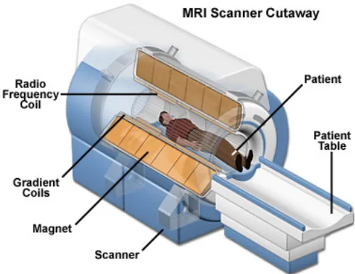
PET [11]. However, there are basic hardware requirements in MRI devices. First and foremost,
it should have a magnet capable of having high magnetic field strengths. This magnet acquire
its strength by an external power supply. Next, it should contain a gradient coil that can
pro-duce a field gradient. The gradient coil propro-duces a secondary magnetic field when the current
passes through it, which will distort the main magnetic field. This allows the spatial
identifi-cation of the MR signal. Furthermore, there should be a radio frequency coil that can transmit
and receive radio frequency oscillations, and a computer to acquire signals and compose the
MR images [12]. A schematic diagram of these components in an MRI device is shown in
Figure 2.2: Main components of an MRI system. Image courtesy of the National Magnetic
Field Laboratory [2]
The MRI signal is generated from the highly abundant protons in brain tissues in the form
of water or fat. Depending on the amount of protons in the tissue, the strength of the MR signal
varies. In the absence of a magnetic field, the magnetic moments of these protons are randomly
oriented. When a strong magnetic field is applied, they interact with the applied field and
par-tially align with the field behaving like tiny bar magnets. Due to this alignment, a small amount
of magnetization is created. Then using a radio frequency signal, a perturbation is introduced
to these protons and when it is removed, the protons will take some time (relaxation time) to
reposition. In the meantime, the observed magnetization will vary and it will gives rise to a
detectable signal in the MRI device. If the relaxation time is long, then the MR signal will be
strong and it will be weak otherwise.
The MRI technique was extended to fMRI in order to obtain information about the
biolog-ical functions of the brain in the 1990s [13]. The basic principle of the fMRI is defined as the
there is neuronal activation in the brain, the blood flow into that activated area increases as
de-manded by neurons to supply energy [14]. The energy needed is provided by supplying more
oxygenated blood. Thus, when a set of neurons activates, more oxyhaemoglobin (which is
diamagnetic) is delivered than deoxyhaemoglobin (which is paramagnetic). Oxyhaemoglobin
can be magnetized by applying an external magnetic field, in the same direction as the external
field (diamagnetic), and deoxyhaemoglobin can be magnetized by applying an external
mag-netic field, in the opposite direction of the external field (paramagmag-netic). Thus, the increase
of oxyhaemoglobin concentration will reduce the local magnetic field with a corresponding
increase in the MRI signal [15].
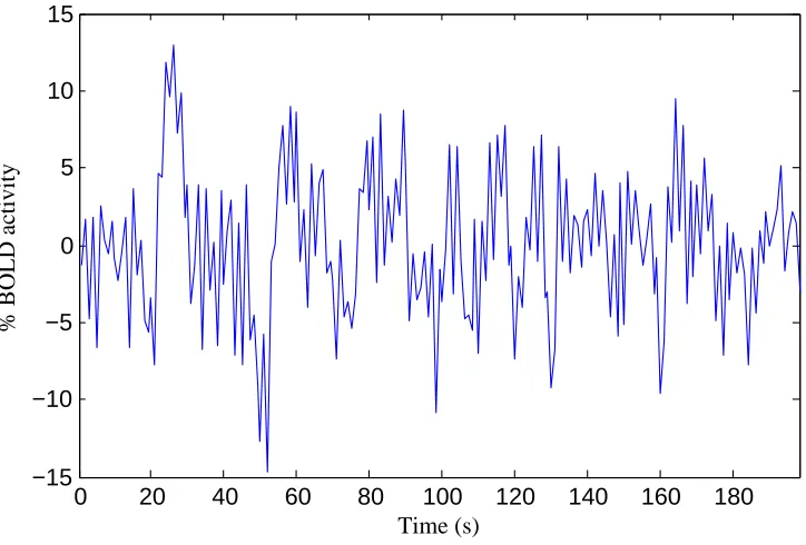
When the imaging techniques are being used, first the brain is divided into voxels, and data
are recorded for each of these voxels. There are millions of neurons in each of the voxels that
are collectively responsible for the observed BOLD signal. This signal oscillates with time as
shown in Figure 2.3. This particular time course was acquired from a brain at rest where the
0 20 40 60 80 100 120 140 160 180 −15
−10 −5 0 5 10 15
Time (s)
% BOLD activity
Figure 2.3: BOLD time course of a patch of cortex from a brain at rest.
2.3.2
Di
ff
usion Tensor Imaging (DTI)
With the advent of MRI, brain imaging has benefited from sophisticated technologies. Imaging
techniques have been developed with more research and, in 1994, the first measurement of the
diffusion tensor in the human brain was made [16]. Following that finding, Diffusion Tensor
Imaging (DTI) was developed step by step to the point that now axonal fibers can be tracked
in the human brain in an accurate manner. DTI is considered a very reliable method to observe
the micro-structural changes in the brain, and it is becoming a popular technique because of
its high sensitivity to the changes at that level. However, there is continuous development to
increase the accuracy and the spatial resolution of DTI.
The fundamental principle behind DTI is the measurement of diffusion (the microscopic
random movements) of water molecules along the axonal fibers in the brain. Diffusion of
bodies, and 50-75% of the volume of our bodies is made up of water, reaching 75% in the
brain. This huge amount of water is distributed in blood, bones and tissues in the body, but
the amount of water the bones have is much less than that in blood or tissues. Due to the high
abundance of water in tissues, it is a helpful substance to track down information about the
micro-structure of the human body.
Water molecules diffuse as a result of thermal fluctuations. This diffusion is stimulated
by an applied magnetic field gradient and at the same time by interactions with neighbouring
molecules or atoms as well as interactions between molecules and cell membranes.
Addition-ally, it is influenced by the structure of these cells containing water [17]. As diffusion depends
on the structure, it is possible to visualize the diffusion of water inside the axons as well as
along the fibers, giving us the opportunity to track down the path of diffusion. White matter
is one type of matter in the brain which is made up of the axons of neurons in which water
molecules can diffuse more freely along the fiber than across the fiber. Thus, the studies of
diffusion in white matter will result in white matter tracts or fiber pathways. This kind of
re-sult could provide valuable information about the biological micro-structures of the brain [17].
Out of the several techniques available, one of the most commonly used DTI technique is
pulsed-gradient, spin-echo pulse sequence, echo-planar imaging [18]. It is an MR technique
that uses an additional magnetic field gradient. As described in the previous section, a strong
homogeneous magnetic field is applied continuously to acquire the MR image. In DTI, the
homogeneity of the magnetic field is disturbed using two magnetic field gradients of opposite
directions, applied one after the other with a time delay. When the first linear magnetic field
gradient is applied, the precession frequency of the protons will change depending on the
mag-nitude of the magnetic field gradient. When it is removed, protons will have different phases.
Then the next magnetic field gradient is applied with the same magnitude but in the opposite
the protons’ movement is restricted, the second gradient will allow them to be refocused to the
same phase again. Thus the produced MR signal will be strong. However, if the water diffuses
in this time gap, the second gradient will not be able to restore the phase shifts that have been
created by the first gradient. Thus, it will produce a weak MR signal [19]. To produce a
com-plete signal using this technique, the diffusion gradient is applied to all the x, y and z directions
in DTI. Afterwards, applying the fiber tractography [20] technique to this diffusion data, the
details about the physical connections in the micro-structure of the brain could be extracted.
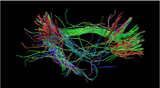
Figure 2.4 indicates the fiber tract orientation of the default mode network of the brain.
Figure 2.4: Lateral view of the white matter tracts in the brain, created by DTI. The colors, red,
blue and green represent the fibers along the x, y and z directions respectively in the cartesian
coordinates (DR Paula et al. in prep.)
2.4
Modelling the Brain
2.4.1
Kuramoto Model
The Kuramoto model was introduced by Yoshiki Kuramoto and used to model the
states lie in the path of a circle where the phase is a variable. The model considersN number
of coupled phase oscillators with natural frequencies distributed in space with a defined
prob-ability density. The model considers two states, synchronized and anti-synchronized states.
In the synchronized state, all the phase oscillators, oscillate with the same frequency and in
the anti-synchronized state, they oscillate with different frequencies. The objective of the
Ku-ramoto model is to explain how the synchronized state and the anti-synchronized state of these
phase oscillators can be distinguished starting with a group of unsynchronized phase
oscilla-tors. These oscillators try to oscillate with their natural frequencies, but the coupling between
them always trys to synchronize the oscillations [22]. The globally coupled oscillators are
defined in the model using equation 2.1:
˙
θi =ωi+
K N
N
X
j=1
sin(θj−θi) (2.1)
whereθi(˙θi) andωiare the phase (rate of change of the phase) and the natural frequency of the
ith oscillator respectively, andN is the total number of oscillators in the system, whileK is a
constant related to the coupling in the system. There are some assumptions in the analysis of
the Kuramoto model which are:
1. All the oscillators are globally coupled (each oscillator affects every other oscillator).
2. Oscillators are identical except for their different natural frequencies [23].
Using this model, it has been found that there is a critical value for the coupling in the
system, and this critical value Kc, is such that forK < Kc the probability of the system being
synchronized is much less and whenKincreases past theKcthe number of oscillators
synchro-nized increases until all of them are synchrosynchro-nized [24]. This critical value was able to identify
a transition between an unsynchronized state and a synchronized state. However, the critical
coupling constant depends on the distribution of the natural frequencies of oscillators, which
Nevertheless, the Kuramoto model has provided a mathematical basis to model some
im-portant phenomena in real life, like simulations of neurons in the brain by modeling the
ob-served oscillations in the BOLD signal. It is used to study some behavioural aspects of neurons
because of the limited variability of the states it has. Additionally, a synchronized behaviour
was also observed in neurons in the brain [25], which motivates the use of the Kuramoto model
to describe the synchronization phenomena in the brain. However, the outstanding problem is
that the model talks about a system that has a constant coupling parameter together with
sinu-soidal phase oscillations as is stated under the assumptions above. In addition to that, according
to the Kuramoto model, the natural frequencies of the oscillators follow the same distribution
all the time, which might not be applicable to the neural activations of the brain.
Generalized Kuramoto Model
Since the Kuramoto model was first introduced, it has been used in several areas of research,
including studying biological systems like the brain. When using the Kuramoto model to model
the dynamics of the brain, Deco and his group introduced some advancements to generalize the
model in order to better capture the effects of structural connectivity in the brain [26]. Two
changes they introduced to overcome the above indicated drawbacks and to generalize the
Kuramoto model were:
1. The coupling strength between each pair of oscillators was extracted using the white
mat-ter tracks of the brain. In other words, it was extracted from the structural connectivity
of the brain instead of being considered a constant.
2. The time delays of the oscillators were being scaled using the structural distance between
the corresponding regions of the brain.
By applying these changes to the original Kuramoto model, Deco et al. generated a
isolated from the brain. Thus modelling the brain dynamics using the generalized Kuramoto
model became more relevant.
2.4.2
Ising model
Two dimensional (2D) Classical Ising Model
The classical Ising model was introduced by Wilhelm Lenz in 1920. The 1D Ising model was
solved by his student, Ernest Ising, in 1925, and the 2D Ising model (in the absence of an
exter-nal magnetic field) was solved by Onsager in 1944 [27]. The 2D Ising model was introduced to
explain the interactions of magnetic spins mathematically. The physical system (a magnet) is
represented by a lattice configuration in the Ising model. Each lattice site has a spin ’s’ which
could take only two possible values, either up (+1) or down (−1) (Figure 2.5). Thus, it is a collection of +1 and −1s representing the spins. This configuration is kept in a thermal bath of temperature T. Interactions between the spins are always influenced by this temperature and
allow the system to reach an equilibrium energy state while resulting in different equilibrium
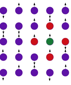
Figure 2.5: Representation of a two-dimensional lattice arrangement. Each lattice site has a
spin, either up or down. The nearest neighbours of the lattice site in green are represented in
red.
The energy of this spin system at any state xin the absence of an external magnetic field
can be calculated using Equation 2.2:
E(x)=−J
N
X
i,j=nn(i)
sisj (2.2)
whereJis the coupling constant,siandsjrepresent the spins of theithand jthsite respectively,
and N is the size of the lattice. For the calculation of energy in the Ising model, only the nearest
neighbour interactions are considered together with equal coupling (J=1). The probability of
finding the system in the statexwith energyE(x)is given by Equation 2.3:
P(x)= 1
Z e
−E(x)
kBT (2.3)
wherekBis the Boltzmann constant,T is the temperature of the heat bath andZ is the partition
function. Equation 2.4 illustrates the partition function of the system which describes the
all possible 2N spin configurations.
Z= X
{x}
e
−E(x)
kBT (2.4)
When a 2D lattice configuration is considered, there are two extreme equilibrium
configura-tions of spins it can hold, one for lower temperatures and the other one for higher temperatures.
When the temperature is very low, all the spins can be aligned along the same direction, with
very large clusters of the same spin, either up or down (ordered) resulting in high
magnetiza-tion even in the absence of an external magnetic field (Figure 2.6 (a)). In the other end, when
the temperature is very high, the spins are a mixture of up spins as well as down spins
(disor-dered) without any order which will result in zero magnetization (Figure 2.6 (c)). In between
these two extremes of temperature, there exists a critical temperature (Tc) [3] where the system
exhibits transition from ordered phase to the disordered phase (Figure 2.6 (b)). As the figure
illustrates, at this temperature there is a mixture of ordered spins as well as disordered spins.
Additionally, the system acquires its maximum susceptibility or the maximum change in
mag-netization atTc. Even a single spin flip can change the entire system [28], and the perturbation
introduced by a single spin flip can spread over the entire system rapidly. Therefore, with
dif-ferent temperatures of the heat bath, the system could exhibit completely different properties
Figure 2.6: Representation of the equilibrium spin configuration for (a)T <Tc, (b)T =Tcand
(c)T > Tc for a two-dimensional lattice arrangement. Red color is for the up spins (+1) and
blue color is for the down spins (−1) [3].
To simulate the dynamics of the classical Ising model, the Metropolis Monte Carlo
algo-rithm is used. The Metropolis algoalgo-rithm involves the construction of a new state based on the
current state of the system with a transition probability. It is used in the Ising model to find
the equilibrium energy state starting from a random spin configuration for a constant
tempera-ture. Monte Carlo simulations are used to describe or to solve systems which change in time
without any predefined dynamical pattern but depending on random numbers created along the
simulations [29]. These algorithms are used in the classical Ising model with the periodic
boundary conditions. Periodic boundary conditions were introduced to the system to restrain
the finite size effects. The application of these algorithms in order to construct the equilibrium
spin states, and then the time fluctuations of the spins for a range of temperatures, will be
dis-cussed in detail in the methodology section (Chapter 3).
An important question that arises next is why it is possible to use the dynamics of the Ising
model which were introduced by using the Metropolis Monte Carlo algorithm to explain the
dynamics of the brain. In the simplest way, spins of the Ising model can be considered as
equivalent to the BOLD activity in the brain with+1 for the activity higher than the baseline
sim-ple model that explains the phase separation. Furthermore, Fraiman et al. [30] state the Ising
model can be used to explain the behaviour of the brain at the critical temperature because of
the similarities it has shown in its dynamics and the brain’s spatio-temporal patterns. The
clas-sical Ising model exhibits long range correlations at the critical temperature, which explains
the observed interactions of the spins that are spatially distant from each other. This fact can be
compared with the functional integration observed in the brain. The brain maintains a balance
between the functional integration and segregation in order to perform efficiently. As observed
in the behaviour of the brain, there are separate regions which are specialized to perform certain
functions. While functioning separately, these regions need to exchange information with each
other in order to function as a complete system. This process is explained as the functional
integration and can be compared with the long range correlations observed in the Ising model.
Thus the classical Ising model was chosen to model the oscillations observed in BOLD signal
for comparison.
Generalized Ising model
The generalized Ising model is an advancement from the classical Ising model. The
general-ization was performed by including the information related to the structure of the brain in the
classical Ising model following the work of Marinazzo et al. [31]. They implemented the
gen-eralized Ising model by using the structural connectivity of the brain, without introducing the
dynamics to the spins variables. By analysing the results they claimed that, the total
informa-tion transfer between spin variables in the model is maximized at the critical state. Similarly,
we implement the generalized Ising model using the structural connectivity; but in addition, we
introduce the dynamics to the spins using the Metropolis Monte Carlo algorithm. The
method-ology will be discussed in details in Chapter 3. However, there are two differences between the
1. According to the generalized Ising model, all the lattice points are interacting with all
the other lattice points with different strengths. This is true in the sense of the structure
of the brain. In the brain, there are some regions that are highly structurally connected
with larger numbers of fibers and some regions that are poorly connected.
2. When using Equation 2.5 to calculate the energy of the system, normalized structural
information is used for Ji j instead of equal coupling as in the classical Ising model
(ex-plained in detail in Chapter 3). Due to this modification, the strength of connection held
between two regions is taken into account by the generalized Ising model.
These two points are illustrated in Equation 2.5:
E(x)= −
N
X
i,j;i,j
Ji jsisj (2.5)
where Ji j is the coupling constant between theithsite and the jthsite. The summation is over
all the sites, without the restriction of the nearest neighbour coupling as in the classical Ising
model.
However, due to these two modifications, the spin sites in the generalized Ising model has
a one-to-one relationship with the patches of cortices in the brain. Hence, it could be used to
study the dynamics of the brain not only on a global level, but also on a local level.
Neverthe-less, the classical Ising model, as described earlier, is a 2-dimensional model, and each spin site
has four nearest neighbours. But in the generalized Ising model, we propose that each region
is connected with every other region, resulting in each site having n 1 (number of regions
-1) nearest neighbours. This makes the model more realistic because, as it is understood from
the structural connectivity data of the brain, there are connections between most of the regions
and not just between the nearest neighbours. Notice that, the dimension of the generalized
critical exponents could be studied at the criticality.
All the observables in the classical Ising model behave according to the Equation 2.6 when
reaching the critical temperature, as explained by Lilian and Manuel in [32]:
O(T)∝| T −Tc
Tc
|α (2.6)
where O(T) is any observable, α is the critical exponent and Tc is the critical temperature.
Thus, we could find the critical exponents for all the observables, such as the magnetization,
magnetic susceptibility, specific heat, correlation function and correlation length. Those critical
exponents should follow the scaling relations given in Equation 2.7 as described in [32]:
(2−η)ν =γ ν
2(η+d−2)=β 2−νd= α
(2.7)
whereβ, γ, α, η, νare the critical exponents of magnetization, magnetic susceptibility, specific heat, correlation function and correlation length, whiledis the dimension of the system.
There-fore, by extracting the critical exponents of the generalized Ising model, we will be able to find
the dimensionalitydof the generalized Ising model (Das et al., in prep.) using the above
scal-ing relations.
2.4.3
Generalized Kuramoto Model versus Generalized Ising model
As explained in the previous sections, the Kuramoto model takes a network of coupled
oscil-lators into account and finds a critical point in between the unsynchronized and synchronized
states of these coupled oscillators. The Ising model takes a spin configuration into account and
disor-dered phase. Both of these phenomena at the critical states are compared with the dynamics of
the brain even though there is no one-to-one relationship between either of the oscillator or the
spin lattice sites and the position of the patch of cortex in the brain.
Sometime after the introduction of the Kuramoto model, it was generalized such that the
coupled oscillators represent the structural regions of the brain, as described in section 2.4.1.
The generalized Kuramoto model could give a detailed explanation of the functional networks
of the brain, starting with the structural connectivity [33]. However, as Deco et al. [26]
explained in the paper, the generalized Kuramoto model still has four main free parameters,
which are mean delay, global coupling strength and two standard deviations from two
Gaus-sian distributions (one modelled for the dispersion of oscillation frequencies and the other one
modelled for the noise of the local networks). Similarly, we are generalizing the Ising model
using the anatomical structure of the brain in place of the constant coupling in the classical
Ising model; but the model has only one controlling parameter, the temperature of the heat
bath.
2.5
Graph Theory
Graph theory is a mathematical tool that can be used to study networks with complex
topolo-gies. It reveals important information about the connectivities in terms of single units and sub
groups as well as a complete network. Graph theory has been used broadly to study highly
complex networks like the internet and air craft flight patterns as it is a simple tool, which
ex-plains the complexity of the subjected networks. Therefore, we use graph theoretical analysis
of the complex brain network. In this context, a graph is a network with source nodes and
edges that connect the nodes. Using graph theory to analyse the complex network of the brain
simplifies the analysis and provides a more general understanding. As Bullmore and Sporns
well handled by the use of graph theory. The equivalent of an edge in a graph could be
ex-plained by a structural or functional connection in the brain network and a node by a region or
a collection of regions in the brain. There are several measures in graph theory being used to
study this complex connectivity.
The degree of a node in the network is one of the simplest measures. It is defined as the
number of links a node has and can be calculated using Equation 2.8:
ki =
X
jN
ai j (2.8)
whereki is the degree of theith node, N is the number of nodes in the network andai j is the
connection status between theith node and the jth node (it is equal to 1 if the nodes are
con-nected and 0 if they are not, in a binary network) [35]. The degree averaged over all the nodes
is defined as the global degree of that network. An understanding about how dense or sparse
the network is could be gained from the average degree of the network.
Following that, we calculated the efficiency for these networks, which is discussed as a
measure of functional integration. The global efficiency of a binary network can be calculated
using Equation 2.9:
EFF = 1
n X
iN
EFFi =
1 n
X
iN
P
jN,j,idi j−1
n−1 (2.9)
where EFFi is the local efficiency, di j is the shortest path length between nodes i and j and
n is the total number of nodes in the network [36]. The efficiency of a network provides an
understanding about the information propagation through the network, or in other words, the
Equation 2.10 was used to calculate the small-world property for each network:
S = C/Crand
L/Lrand
(2.10)
whereC andCrand are the clustering coefficients, and L and Lrand are the characteristic path
lengths of the network being tested and a random network respectively. A random network
is created by preserving the degree distribution of the tested network. Small-world networks
are characterized by the average short path lengths and high clustering coefficients [37]. It
is a measure of the balance between information integration and segregation. Average path
length is a measure of integration which is defined as the average of shortest distance between
each pair of nodes. Clustering coefficient is a measure of the segregation or in other words it
measures the tendency of the nodes to cluster together. In neuroscience, it has been shown in
several analyses that the brain network shows small-world network properties, implying that
it maintains a balance between integration and segregation. Small-world networks often have
values greater than 1 forS [38, 35]; but the value ofS could easily be misinterpreted without
knowing about the connectivity of the network. For an example, the average path length can be
very small for networks with lower number of edges and lower number of participating nodes.
Although the clustering coefficient can be high for these type of networks because of the small
number of nodes in the network. This can result in higher small-world property which stands
Methodology
3.1
Overview
In this chapter, we focus on the procedure for generating the two types of data sets we used:
brain data and simulations. In the first section, we would like to focus on the method of
ex-traction of the functional brain data from fMRI. The methodology used for the acquisition and
extraction of structural data using DTI will then be explained, followed by a section with a
de-tailed explanation of numerical simulations of the models. The acquisition and preprocessing
of fMRI data and DTI data was performed by Erik Ziegler (University of Liege, Liege,
Bel-gium). In section 3.3, we will describe the methodology for the simulation of the generalized
Ising model. The simulations of the classical Ising model will be described after that followed
by a description of the methodology used for the analysis of these data.
3.2
Empirical Data from MRI
3.2.1
Subjects
For the collection of data, 14 healthy subjects with mean age 43±15 were studied, including seven women. The study was approved by the Ethics Committee of the Medical School of the
University of Liege. In addition, informed approval to participate in the study was obtained
from all the subjects. From these healthy subjects, the resting state fMRI (rsfMRI) and DTI
data were acquired and preprocessed using the methods described below.
3.2.2
Acquisition & Preprocessing
Functional Data
Resting state BOLD data were acquired on a 3-T MR scanner with a gradient-echo echo-planar
imaging sequence using axial slice orientation and covering the whole brain (32 slices, voxel
size: 3 × 3 × 3mm3; matrix size 64 × 64 × 32; repetition time = 2000ms; echo time = 30 ms; flip angle=780). Data preprocessing was performed using Statistical Parametric Mapping
(SPM) 8 (www.fil.ion.ac.uk/spm). Preprocessing steps included realignment and adjustment
for movement related effects, co-registration of functional images with structural images,
seg-mentation of structural data, spatial and functional normalization and spatial smoothing of the
fMRI data.
Segmentation of images for each subject was performed with the FreeSurfers
Desikan-Killiany atlas [39]. This atlas provides the ability to separate the brain into gyral-based regions
of interest (ROI) automatically. Thus using the atlas, the images could be segmented. Further
parcellation, using the Lausanne 2008 atlas and its 83 individually labelled regions, was done
with functions from the Connectome Mapping Toolkit [40, 41, 42]. The labels of the 83
regions are presented in Appendix C followed by a figure representing the 83 regions (Figure
.3).
Structural Data
Diffusion Weighted Images (DWI) were acquired from each subject, and the Fractional Anisotropy
that, orientation distribution functions were obtained for each voxel. Probabilistic
tractogra-phy [43] was performed throughout the whole brain using randomly placed seeds inside a
subject-specific white-matter mask. The set of points representing each fiber track were then
affine-transformed into the subjects’ structural spaces which results in the connectivity maps.
Finally, connectivity matrices with the number of fibers connecting each of the 83 regions with
all the others were obtained for 14 subjects, and the normalized mean connectivity was used as
an input of the generalized Ising model.
3.2.3
Resting State Network (RSN) extraction
After using Independent Component Analysis (ICA) [44] for BOLD decomposition in an
in-dependent data set of 19 healthy controls, nine Resting State Networks (RSNs) were identified
in each subject, and an average template was created for each RSN. Subsequently, by setting
a separate threshold for each RSN, the region of interests (ROIs) out of the 83 parcellated
re-gions belonging to the network were extracted. Extracted ROIs for each network are presented
in Appendix D. Finally, the lines of the correlation matrix corresponding to each ROI for the
same RSN were averaged in order to obtain the linear-correlation maps plotted in Figure 4.9.
3.3
Numerical Simulations
3.3.1
Generalized Ising Model
The generalized Ising model was developed by starting with a 1D-random spin configuration
of lattice of size 83, which is assumed to be in contact with a thermal bath of temperature T.
The steps below have been followed according to the Metropolis Monte Carlo algorithm to
obtain the equilibrium spin configuration, for a particular temperature starting with random
spin states. The connectivity matrix used for the simulation of the generalized Ising model is
1. A random spin configuration was defined with the lattice size of 83.
2. Initial energyEin of the system was calculated using Equation 2.5.
3. Next, one spin was selected randomly from the spin configuration and was flipped.
4. The new energyEnewwas calculated.
5. ThenEin andEnewwere compared.
• IfEnew < Ein, the spin flip was accepted and the new configuration was considered
the initial configuration withEin=Enew. Then the simulation was continued starting
from Step 3.
• IfEnew > Ein, the Boltzmann factor B=e −∆E
kBT was calculated and a random
num-berrwas drawn from a normal distribution. Then these two values were compared.
– If B > r, the spin flip was accepted andEin was replaced withEnew. Then the
procedure was repeated starting from Step 3.
– If B < r, the spin flip was rejected, and the simulation was started over from Step 3.
The steps starting from Step 3 were repeated until we obtained an equilibrium spin
configu-ration with an equilibrium energy for a particular temperature. At the equilibrium state, energy
of the system fluctuates within a small range. The random configuration can evolve into this
state by following single-spin-flip dynamics as explained in the algorithm. This equilibrium
configuration was considered as the configuration at time t= 0. After that, by following the
Metropolis Monte Carlo simulations, the time evolution of the equilibrium spin configuration
was obtained as follows;
• Next, all the spins in the configuration were tested for flip by flipping one at a time and comparing Ein and Enew to decide whether to accept or to reject the flip using the
Metropolis Monte Carlo algorithm. After all the spins had been checked, the new
con-figuration was considered the concon-figuration at time t=1.
• After that, all the spins of this new configuration were checked for flip as in the previous step. When all the spins had been checked, the new configuration was taken as the
configuration at time t=2.
• These steps were repeated until we found as many time points as needed to compare with the empirical data.
By the end of this process, the time evolution of the spins for each spin site was obtained.
Using these time series data, and Equation 3.1, the correlation between each pair of sites in the
lattice was calculated:
ρi j =
< si(t)sj(t)>− < si(t)>< sj(t)>
σsi(t)σsj(t)
(3.1)
whereρi j is the correlation between theithand jthspin time series,si(t) and sj(t) stands for the
spin time courses of theithand jthregion,σ2
si(t)=< s
2
i(t)> −< si(i)>
2and< . >is the average
over time.
Starting from a random configuration, this complete procedure was repeated for different
temperatures ”T” ranging from 0.5 to 3 in increments of 0.01. Additionally,kB was equated to
one, in the simulations. This was repeated for ten iterations, and data were recorded separately
each time. We performed the simulation for ten iterations to observe the effect of
randomiza-tion of the spins at the first step of the simularandomiza-tions. An illustrarandomiza-tion of the variarandomiza-tion with respect
Figure 3.1: Connectivity matrices used for the simulations of the classical Ising model (a) 9×
9 , (b) 10×10, and (c) the generalized Ising model.
During these simulations, the energy (E), magnetization (M) and susceptibility (χ) of the system were calculated using Equations 2.5, 3.2 and 3.3 respectively at each temperature:
M = 1
N
N
X
i=1
si (3.2)
χ= 1
NT[< M
2 >−<
M>2] (3.3)
where N = 83 and si is the spin of the ith region. Derivation of Equation 3.3 is presented in
[45]. These quantities were plotted as a function of temperature, and the susceptibility versus
temperature plot was used to extract the critical temperature (Tc), which gives the highest
susceptibility. Super critical (T > Tc) and sub critical (T < Tc) temperatures were chosen
relative to the critical temperature. The MATLAB code which was used for the simulations of
the generalized Ising model is attached in Appendix A.
3.3.2
2D Classical Ising Model
The classical Ising model was developed by following the same steps, and using Equation 2.2
nearest neighbour interactions. The 2D Ising model was simulated using two lattice sizes 9×9 (L=9) & 10×10 (L=10) which result in 81 and 100 spin sites respectively. These two sizes were chosen to make the 2D Ising model comparable with the empirical data, which has 83
spin sites. Given this choice, two separate data sets were obtained for each lattice size with
temperature ranging from 0.5 to 4. The connectivity matrix used for the simulations of the
classical Ising model is presented in Figure 3.1 (a) and (b).
In a similar manner, Equations 3.2 and 3.3 were used to calculate the magnetization and
susceptibility of the system, whereN = L×Lin the classical Ising model. After extracting the critical temperature for both of the lattice sizes, those values were verified using Equation 3.4
[32]:
Tc =(20.28)×
1
L2 +2.26 (3.4)
where L is the length of the square lattice (either 9 or 10).
3.4
Comparison of data
As explained in the previous sections, the functional correlation was obtained for the regional
parcellation of 83 regions in the brain using rsfMRI, which will be hereafter called the
empiri-cal data. The structural connectivity was obtained by the extraction of white matter tracts from
DTI. In addition to that, we generated three sets of data from the mathematical simulations of
the Ising model: one from the generalized Ising model using the structural connectivity, and
the other two sets from the classical Ising model for two different lattice sizes.
The mean data over the ten iterations were considered to perform our analysis. A
compar-ison of the correlations of the empirical data, generalized Ising model data and the classical
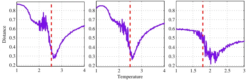
Ising model data was performed first. After observing the correlation maps for three different
to find the temperature which minimizes the distance between two cumulative distributions for
each model. KS test is a non-parametric test which has been used to test two distributions. The
test statistic calculates the maximum distance between two cumulative distributions and this
has been used to find the temperature which minimizes the distance between two distributions
in our data. Thereafter, graph theoretical measures as explained in Chapter 2 have been used
to compare the classical Ising model and generalized Ising model data with the empirical data.
Results
4.1
Overview
In this chapter, we will present our results obtained using the methodology explained in Chapter
3.
4.2
The Classical Ising model versus the Generalized Ising
model
Three correlation data sets were obtained by following the procedure explained in Chapter 3.
During the process of creating these, the energy, magnetization and susceptibility of the
sys-tems were calculated as a function of temperature. Hence, these quantities were plotted for the
classical Ising model, as well as for the generalized Ising model, as shown in Figure 4.1.
1 2 3 4 0 0.2 0.4 0.6 0.8 1 Magnetization
1 2 3 4
0 0.2 0.4 0.6 0.8 1
0.5 1 1.5 2 2.5 3
0 0.2 0.4 0.6 0.8 1
0.5 1 1.5 2 2.5 3
0 0.05 0.1 0.15 0.2
0.5 1 1.5 2 2.5 3
−1 −0.8 −0.6 −0.4 −0.2 0
1 2 3 4
0 0.05 0.1 0.15 0.2 Susceptibility
1 2 3 4
0 0.05 0.1 0.15 0.2
1 2 3 4
−1 −0.8 −0.6 −0.4 −0.2 0 Energy
1 2 3 4
−1 −0.8 −0.6 −0.4 −0.2 0 Temperature
(a) (b) (c)
Figure 4.1: Magnetization, susceptibility and Energy as a function of temperature for the
Clas-sical Ising model with (a) 9 × 9 and (b) 10 × 10 lattice size, and (c) the Generalized Ising model. Red dashed line indicates theTc.
The critical temperature was extracted in both models using the susceptibility versus
tem-perature plot (second row of the Figure 4.1). Relative to the critical temtem-perature, a sub-critical
and a super-critical temperature was selected such that for both of the models the selected
tem-peratures maintain the same distance with the critical temperature (Table 4.1).
Model T <Tc T =Tc T > Tc
Generalized Ising model 0.64±0.06 1.79±0.06 2.89±0.06
Classical Ising model (9×9) 1.40±0.10 2.55±0.10 3.65±0.10 Classical ising model (10×10) 1.35±0.06 2.50±0.06 3.60±0.06
Table 4.1: Extracted temperature values for the three cases in the two models
Carlo Algorithm, and used to calculate the correlations among the spin sites. An illustration
of the correlations relative to the extracted three temperatures is presented in Figure 4.2 for the
classical Ising model and for the generalized Ising model.
Figure 4.2: Correlation atT <T c,T =T c, andT > T cfor the classical Ising model with (a) 9
![Figure 2.1: Main components of a neuron [1]](https://thumb-us.123doks.com/thumbv2/123dok_us/7741110.1268008/18.612.213.392.73.300/figure-main-components-of-a-neuron.webp)