Contribution to the Analytical Evaluation of the Efficiency and the
Optimal Control of Conductive Fluids by Electromagnetic Forces
Hocine Menana1, * and C´eline Gabillet2
Abstract—This work deals with the evaluation of the efficiency and optimal control of conductive fluids by using electromagnetic forces. An electromagnetic actuator based on a succession of electrodes and magnets annuli is implemented on the surface of the rotating cylinder of a Taylor-Couette device. Considering a laminar flow, the magnetohydrodynamic (MHD) problem is formulated and solved analytically. The different MHD powers, control efficiency and optimal values of the control parameters are evaluated.
1. INTRODUCTION
Depending on the possibility of use, several passive and active techniques can be used to control the fluid flow boundary layers in order to prevent flow separation, and to reduce the drag and losses [1–6]. For conductive fluids, electromagnetic forces can be used. Structures of electromagnetic actuators formed by electrodes and magnets have been developed to create Lorentz forces parallel or perpendicular to the fluid flow [2–6]. However, low efficiencies are obtained due to the weak electrical conductivity of common fluids. In order to optimize such control, an explicit expression of the efficiency with respect to the physical and geometrical properties of the system is necessary. In this context, the aim of this work is to provide an analytical expression of the electromagnetic control efficiency as function of the physical and geometrical properties of the system.
The fluid control is considered in a Taylor-Couette device [6]. An annular structure of an electromagnetic actuator constituted of an array of electrodes and magnets [2, 3] is implemented on the surface of the rotating cylinder. The expression of the Lorentz forces is adapted to take account of the annular form of such actuator, through the expression of the variations of the electrical current and magnetic flux densities with respect to the radial direction. Considering laminar flows, the MHD problem is formulated and solved analytically. The different MHD powers are evaluated. The optimal control, defining the value of the applied electrical current density that minimizes the total MHD losses in the system, is studied.
The modeled system and the problem formulation are presented in the next section. Results and discussions are given in the last section.
2. MHD MODEL FORMULATION
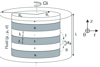
The modeled system is shown in Fig. 1. An electrically conductive fluid is contained between the inner and outer cylinders of a Taylor-Couette device. An electromagnetic actuator based on a succession of electrodes and magnets annuli of equal widths, creating wall parallel Lorentz forces, is implemented on the surface of the inner cylinder which is rotating at a radial speed Ωi while the outer cylinder is
Received 10 January 2017, Accepted 23 March 2017, Scheduled 2 April 2017
* Corresponding author: Hocine Menana ([email protected]).
1 GREEN Research Group, Lorraine University, Campus Aiguillettes, BP 70239, Vandoeuvre-Les-Nancy 54506, France. 2 French
Figure 1. The modeled system.
at rest. As shown in Fig. 1, Ri and Re are respectively the outer and inner radii of the inner and outer cylinders,λis the electrodes and magnets annuli width,J is the current density on the electrodes surfaces, and B0 is the magnetic flux density on the magnets surfaces. The Taylor-Couette device is
considered infinitely long (i.e., LRe−Ri), so as the end effects (interaction of the fluid with the end walls) can be neglected.
The electrical current density on the electrodes surface depends obviously on the fluid conductivity. As in the presented model, we apply a current source rather than a voltage source, the electrical current density is forced to a certain value (J) in the electrodes surfaces regardless the fluid conductivity. In practice, this is achieved by adapting the voltage magnitude between the electrodes to the electrical resistivity of the fluid to obtain the desired value of the electrical current density. This is why the fluid conductivity does not directly appear in certain parts of the model presented below, such as in the equation giving the electromagnetic power transmitted to the fluid by the Lorentz forces which depends directly on the electrical current and magnetic flux densities. However, the Joule losses and thus the control efficiency depend on the electrical conductivity of the fluid which is directly involved in the corresponding equations.
2.1. The Electromagnetic Forces Created in the Fluid
In the condition where λ (Re−Ri), the Lorentz forces created by the actuator in the direction of the fluid flow (θ) is given by Eq. (1). It is an adaptation of the expression of the force produced by a planar structure of such actuator [2, 3], tacking account of the variations of the electrical current and magnetic flux densities with respect to the radial direction, which is represented by the term f(r).
F(r) = π
8J B0exp
−π
λ(r−Ri)
×f(r)|r∈[Ri,Re] (1)
The function f is related to the ratio between the surface (SRi) of the inner cylinder of radius (Ri) and the surface (Sr) of a fictitious cylinder of radius (r =Ri+ Δr) between the inner and outer cylinders. The relation between Sr and SRi is:
Sr=SRiRi−1r =SRi1 +R−i 1Δr. (2)
In the case where Δr Ri, we can write:
Sr≈SRiexp(Δr/Ri) =SRiexp(r/Ri−1). (3)
The magnetic flux and current densities decrease thus with a factor 1/exp(r/Ri−1). As the force is proportional to the product of these two quantities, it decreases with the square of this factor, and thus we obtain:
f(r) = exp(−2r/Ri+ 2). (4)
2.2. The MHD Problem Formulation
Neglecting the end effects and assuming a laminar flow, the magnetohydrodynamic problem formulation is given in cylindrical coordinates (r, θ, z) by Eq. (5). It is derived from the Navier-Stokes equation in which we consider only the azimuthal fluid velocity (u) variation with respect to the radial directionr, i.e., ∂θu= 0 and ∂zu= 0, where ∂θ and ∂z denote the derivatives with respect to θ and z. In Eq. (5), ρ and μare the fluid density and dynamic viscosity.
ρ ∂tu−μ(∂2
ru+r−1∂ru−r−2u) =F(r)
u(Ri) =RiΩi, u(Re) = 0 (5)
Notice that there is no variation of the magnetic field with the fluid motion in the azimuthal direction, and thus no eddy currents are created in the fluid due to the rotation. Indeed, as shown in Fig. 2, any closed circuit (Γ) moving in the azimuthal direction would be crossed by the same magnetic flux, and thus: dφ/dt= [dφ/(rdθ)]×[rdθ/dt] =u×dφ/(rdθ) = 0.
Figure 2. Illustration of the cancellation of the induced currents in the fluid.
In the steady state regime (∂tu= 0), Equation (5) becomes:
∂r2u+r−1∂ru−r−2u=−aexp (br+c) (6)
where: a= 0.125πJ B0μ−1,b=−(πλ−1+ 2R−i 1) and c=πRiλ−1+ 2.
The solution of Eq. (6) is given as follows:
u=r−1(b2r2−c2)C1+C2−ab−3(br−1) exp (br+c)
. (7)
With the boundary conditions given in Eq. (5), we obtain:
⎧ ⎪ ⎨ ⎪ ⎩
C1=
ΩiR2
i −ab−3
(bRe−1)ERe−(bRi−1)ERi b2(R2
i −Re2) C2=ab−3(bRe−1)ERe−(b2Re2−c2)C1
(8)
In (8): ERe = exp(bRe+c) and ERi = exp(bRi+c).
If no electromagnetic forces are applied, i.e., F = 0, the solution (u0) of Eq. (5) becomes [7]:
u0 =Ar+Br−1, where, in this case, A= ΩiR2i(R2i −Re2)−1 andB = ΩiR2i.
2.3. The System Power Evaluation
The total MHD power (PMHD) is the sum of the Joule power losses in the fluid (PJ), the electromechanical power transmitted to the fluid by the Lorentz forces (Pem), and the friction power (Pμ) due to the fluid viscosity [8].
PMHD =PJ+Pem+Pμ (9)
As the outer cylinder is at rest, the energy loss due to friction in the fluid is the energy given to the flow by the inner cylinder [10]. The force applied on the inner cylinder is due to the fluid viscosity creating shear stress τ =μ(∂ru−r−1u) on its surface (Si) [9, 10]. The friction power loss can thus be evaluated as follows:
Pμ=
Si
μu(∂ru−r−1u)r=R
ids= 4πLμΩi
c2C1−C2−ab−3(0.5b2R2i −bRi+ 1)ERi
If no electromagnetic forces are applied, the friction power loss becomes:
Pμ0 =−4πLμRiΩ2i (11)
The Joule losses in the fluid can be expressed as follows, whereσ is the fluid electrical conductivity, Jf is the electrical current density in the fluid, andLis the axial length of the inner and outer cylinders. The negative sign denotes losses.
PJ =−2πLσ−1
Re
Ri
Jf2(r)rdr=−π2LJ2(4σb2)−1(bRe−1)ERe−(bR
i−1)ERi (12)
The electromechanical power transmitted to the fluid by the Lorentz forces is given by Eq. (12). It involves only the fluid velocity induced by the electromagnetic forces [8], which is taken into account directly by setting Ωi = 0 in the integration coefficients of Eq. (8).
Pem = 2πL
Re
Ri
F×u(Ωi=0)rdr=J2B0Lπ2(4b)−1×
C10(b2r2−2br−c2−2) +C20
exp (br+c) +a0(4b3)−1(3−2br) exp (2br+ 2c)
Re
Ri (13)
with:
C10=C1(Ωi = 0 and a=a0 = 0.125πB0μ−1)
C20=C2(C1 =C10 and a=a0)
(14)
2.4. The Control Efficiency
The control efficiency is defined as the ratio of the power saved to the power used for the fluid control. In the laminar flow, the electromechanical power transmitted to the fluid is equal to the power saved by friction loss on the cylinder surface [8]; therefore, the evaluation of the control efficiency can be limited to the electromagnetic part (Lorentz forces versus Joule Losses). By writing |Pem|and |PJ|as follows:
|Pem|=Pem=J2B02Lψem(Ri, Re, λ)
|PJ|=−PJ =J2σ−1LψJ(Ri, Re, λ) (15) whereψem and ψJ are positive functions depending only on the geometrical parameters, we have
ηem= P
0
μ− |Pμ| |PJ|+|Pem|=
|Pem| |PJ|+|Pem| =
1 + ψJ σB2
0ψem
−1
(16)
2.5. The Optimal Control
Correctly applied, Lorentz forces tend to accelerate the fluid in such manner to get a compensation of a part of the friction power on the inner cylinder surface. However, this is followed by Joule power losses due to the electrical current flow in the fluid. For a given geometry, the optimal control corresponds thus to the current densityJopt that minimizes the total MHD power in the system.
∂JPMHD =∂JPJ+∂JPem+∂JPμ= 0 (17)
By writing: ⎧
⎨ ⎩
∂JPem = 2J B02Lψem(Ri, Re, λ) ∂JPJ =−2J Lσ−1ψJ(Ri, Re, λ) ∂JPμ=LB0Ωiψμ(Ri, Re, λ)
, (18)
we obtain:
Jopt=B0ψμΩi×[2(σ−1ψJ−B02ψem)]−1 (19)
3. RESULTS AND DISCUSSIONS
For a quantitative study, we set the system parameters to the numerical values given in Table 1. The system parameters are arbitrary chosen but satisfy the condition of a laminar flow. This is verified by the evaluation of the Taylor number T n=Ri(Re−Ri)3μ−2ρ2Ω2i, which must be less than its critical value of about 1700 [7–9].
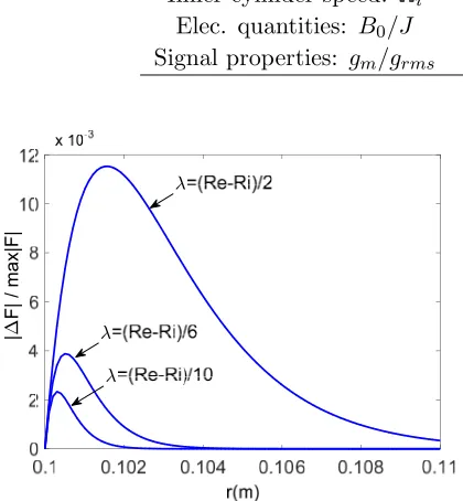
Figure 3 gives the normalized absolute value of the difference between the Lorentz forces obtained by the planar and the corrected models in Eq. (1), for different values of the electrodes and magnets annuli widthλ. As expected, the difference depends strongly on the ratio (λ/Ri). It is relatively feeble, however, for a better accuracy one has to take it into account.
The Lorentz forces can be created either in the direction of the fluid flow to give an additional kinetic energy to the latter or in the opposite direction to reduce the drag caused by the moving cylinder in the fluid, as shown in Fig. 4. The velocity profiles corresponding to opposites values of the current density (i.e., +J and −J) are not symmetrical, which is due to the effect of the inner cylinder velocity. An important result to notice is that we can reduce the section of the fluid flow between the cylinders and thus reduce the value of the Taylor number described above. This will delay the transition of the fluid flow from laminar to turbulent where the hydrodynamic losses are much higher. This is the main purpose of the electromagnetic control.
Figure 5 gives the control efficiency as function of the fluid electrical conductivity for different electrodes and magnets annuli width λ. As expected, the control efficiency increases with the fluid conductivity and decreases dramatically for weakly conductive fluids. Increasing the ratio (λ/(Re−Ri)) leads to an increase of the electromagnetic forces created in the fluid and thus increases the control efficiency. For sea water (σ ≈5 S/m), we obtainηem= 2×10⁻³forλ= (Re−Ri)/2, andηem= 0.9×10⁻⁴
Table 1. Parameters specifications.
Parameters Values
Dimensions: Ri/Re/L/λ 0.1 m/0.11 m/1 m/variable (m) Physical properties: μ/ρ/σ 10−3Pa·s/103kg/m3/variable (S/m)
Inner cylinder speed: Ωi 0.1 rad/s Elec. quantities: B0/J 1 T/variable (A/m2)
Signal properties: gm/grms 1/1 (constant signal)
|
F| / max|F|
Figure 3. The difference between the planar and modified Lorentz forces distributions between the cylinders, for different values ofλ.
Fluid velocity (m/s)
em
Figure 5. The control efficiency as function of the fluid conductivity for different values of λ (J =−100 A/m2).
opt
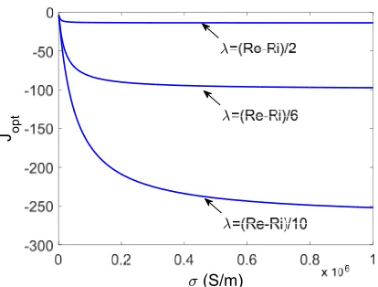
Figure 6. The optimal electrical current density as function of the fluid conductivity (Ωi = 1 Rad/s, B0 = 1 T).
forλ= (Re−Ri)/10.
Figure 6 gives the optimal current density that minimizes the total MHD power in the system, as function of the fluid electrical conductivity, for different values of λ. When the conductivity is feeble, the Joule losses are important and thus the optimal current is feeble. As the conductivity grows, the Joule losses decrease and the optimal current increases to reach to asymptotic value given by Eq. (19). The latter involves the applied magnetic flux density, the inner cylinder speed, the fluid viscosity and the geometrical parameters of the system.
Jopt(σ → ∞)≈ −ψμΩi[B0ψem]−1 (20)
4. CONCLUSION
This work gives an analytical expression of the electromagnetic control efficiency of a conductive fluid in a Taylor-Couette device, as function of the physical and geometrical properties of the system. This explicit expression allows a better understanding of the influence of each parameter and to determine the optimal values of the control parameters.
The electromagnetic control efficiency of common fluids is very feeble in laminar flows; however, it is shown that with such control, one can modify the Taylor number in such way to delay the transition of the fluid flow from laminar to turbulent where the hydrodynamic losses are much higher.
For simplicity, an infinite Taylor-Couette geometry is considered in order to neglect the end walls effects. The model can be extended in the laminar regime to the geometries used in experiments by introducing a variation of the fluid velocity according to the axial direction.In this case, induced currents occur in the fluid and they have to be taken into account. Analytical modeling is still possible for small and symmetrical disturbances [7], however, for high Ta numbers, numerical modeling would be necessary, nevertheless, the analytical expression of the electromagnetic force still can be used.
APPENDIX A.
The functionsψμ,ψem and ψJ are given as follows:
ψμ=π2(2b3)−1×b2R2e−2c2(bRe−1)E
Re−(bR
i−1)ERi b2(R2
i−R2e) −
(0.5b2R2i−bRi+1)ERi−(bR
e−1)ERe
ψJ=−π2(4b2)−1(bRe−1)ERe−(bRi−1)ERi
ψem=π2(4b)−1×C100(b2r2−2br−c2−2)+C200
exp (br+c)+a00(4b3)−1(3−2br) exp (2br+2c)
Re
with:
a00= 8πμ, C100 =C10(a=a00), C200=C20(a=a00).
REFERENCES
1. Oualli, H., M. Mekadem, M. Lebbi, and A. Bouabdallah, “Taylor-Couette flow control by amplitude variation of the inner cylinder cross-section oscillation,” Eur. Phys. J. Appl. Phys., Vol. 71, 11102, 2015.
2. Albrecht, T., J. Stiller, H. Metzkes, T. Weier, and G. Gerbeth, “Electromagnetic flow control in poor conductors,” Eur. Phys. J. Special Topics, 220–275, 2013.
3. Berger, T. W., J. Kim, C. Lee and J. Lim, “Turbulent boundary layer control utilizing the Lorentz force,”Physics of Fluids, Vol. 12, No. 3, 631–649, March 2000.
4. Weier, T., U. Fey, G. Gerbeth, G. Mutschke, O. Lielausis, and E. Platacis, “Boundary layer control by means of wall parallel Lorentz forces,”Magnetohydrodynamics, Vol. 37, No. 1–2, 177–186, 2001. 5. Hinze, M. “Control of weakly conductive fluids by near wall Lorentz forces,”GAMM-Mitt, Vol. 30,
No. 1, 149–158, 2007.
6. Thibault, J.-P. and L. Rossi, “Electromagnetic flow control: Characteristic numbers and flow regimes of a wall-normal actuator,” J. Phys. D: Appl. Phys., Vol. 36, 1, 2003.
7. Taylor, G. I., “Stability of viscous liquid contained between two rotating cylinders,” Phil. Trans.
R. Soc. Lond. A, Vol. 223, 289–343, 1923.
8. Menana, H., J. F. Charpentier, and C. Gabillet, “Contribution to the MHD modeling in low speed radial flux AC machines with air-gaps filled with conductive fluids,” IEEE Trans. Mag., Vol. 50, No. 1, Vol. 8100104, 1–4, January 2014.
9. White, M. F., Fluid Mechanics, 4th Edition, McGraw-Hill, Inc., 1995.
![Fig. 2, any closed circuit (Γ) moving in the azimuthal direction would be crossed by the same magneticflux, and thus: dφ/dt = [dφ/(rdθ)] × [rdθ/dt] = u × dφ/(rdθ) = 0.](https://thumb-us.123doks.com/thumbv2/123dok_us/1982565.1262024/3.612.231.388.268.336/fig-closed-circuit-moving-azimuthal-direction-crossed-magneticux.webp)