THE INTERACTION OF SELECTION AND LINKAGE. II. OPTIMUM MODELS

OF

OPTIMUM MODELS1 R. C . LEWONTIN2

Department of Biology, University of Rochester, Rochester, N.Y.

Received June 16, 1964

I N the first paper in this series (LEWONTIN 1964)

I

discussed the consequences of linkage in populations subject to natural selection when there is heterosis (higher fitness of heterozygote than of homozygotes). There is a great deal of theoretical and experimental evidence concerning the existence of heterosis at the level of single loci (so-called ouerdominance)

,

but it seems to be as yet un- determined whether such overdominance is widespread or only of academic interest

.

On the other hand, there can be no doubt at all that “optimizing selection” must be an extremely common and important biological phenomenon. By “opti- mizing selection” I mean that in a continuum of possible phenotypes, there is some intermediate value which has the greatest selective advantage and that deviations on either side of this intermediate phenotype are less fit on the average.

It is a commonplace that there is a relatively narrow range of optimal size for a n animal and although there is considerable genetic variation for size in both directions in a population of say, Drosophila, the population tends to remain at an intermediate phenotypic level. Even a component of fitness like fecundity can be increased over its normal value by artificial selection (KOJIMA and KELLE- HER 1963) so that correlation with other fitness components somehow holds fecundity at an intermediate value in natural populations.

Even though the widespread existence of “optimizing selection” cannot be questioned, what is still not thoroughly understood is the extent to which such selection can maintain genetic variation in a population. FISHER (1 930) first alluded to a n optimum selection scheme later more fully developed by MATHER

(1941 )

.

FISHER’S scheme was that there were two factors A , a and €3, b such that “ A is advantageous in the presence of B but disadvantageous in the presence of b, and that B is advantageous in the presence of A but disadvantageous in the presence of a.” Couched, as this description is, in terms of gene advantages rather than diploid genotypic fitnesses, it is not unambiguous in its interpretation and as it stands is neither a sufficient nor necessary description of the kind of two factor interaction necessary for stable equilibrium of gene frequencies and for linkage effects of a permanent sort. In the first careful treatment of a two factor polymorphism, KIMURA (1956) showed, in fact, that in order for the system

This investigation was performed under Atomic Energy Commission Contract AT(30-1)2620. The extra cost of setting

Present address: Department of Zoology, University of Chicago, Chicago, Illinois. tables and formulas, and the page charge has been defrayed by this contract.

described by FISHER to be stable, at least one of the factor pairs would have to be

unconditionally heterotic.

FISHER went further and considered an explicitly optimum model in his dis-

cussion of metrical characters. Here he assumed that the mean of the population was the optimum and that at a single locus the fitness of a genotype fell off with its squared deviation from the mean. FISHER then went on to show that such a system does not lead to a stable equilibrium but that the gene frequencies might be balanced by recurrent mutation and thus account for the observed genetic variability for metric characters. The absolute instability of this model of FISHER’S

arises because fitness falls off with deviation from the population mean and not from a fixed optimum phenotype.

Another treatment of linkage and optimizing selection and one that in some part grew out of FISHER’S earlier suggestion was that of MATHER (1941).

MATHER’S suggestion of “internal” and “relational balance” amounts to a model

in which an intermediate phenotype is most fit for a character determined by a large number of loci of similar small action, “polygenes”. At each of these loci there are plus and minus modifiers of the phenotype and no epistasis is assumed on the primary phenotypic scale. I n general MATHER does not specify how fitness falls off with deviation from the optimum phenotype and the only numerical case he presents of the model (on page 186 of his 1941 paper) does not lead to a stable equilibrium of gene frequencies. Like FISHER, MATHER predicts the buildup of linked repulsion complexes of genes as a result of the optimizing selection, but the models explicitly discussed are not stable. BODMER and PARSONS (1962) present several models based upon the relational balance theory of MATHER,

models that do lead to the predictions made by MATHER. However, all such models have, in addition to the optimality of intermediate phenotypes, an assump- tion of superior heterozygote fitness not obviously related to the phenotypic score. Thus, it is assumed by BODMER and PARSONS that the double heterozygote A a Bb

is more fit than the so called “balanced homozygotes” A A bb and aa BB. More recently PARSONS (1963) tried to relax this assumption of heterozygote superi- ority but the stability, in fact, disappears with the heterosis. In this connection the point made by KIMURA (1956) must be reiterated, that interaction and link- age alone cannot maintain stable gene frequency equilibria and linkage com- plexes. There must be some heterosis of fitness as well. Thus the balance models

of BODMER and PARSONS can be subsumed under the general rule that epistatic

deviations of any kind will lead to the buildup of stable linked complexes when recombination is restricted, provided that each locus shows marginal over- dominance for fitness at equilibrium (KOJIMA 1959a).

WRIGHT (1935) considered a quadratic deviation model in which the fitness

of a phenotype falls off as the square of the deviation of that phenotype from some optimum. WRIGHT showed that if the genes controlling the phenotype have either complete dominance or complete additivity, there could be no stable equilibrium of gene frequencies. Eventually all genes controlling the character would be fixed. Essentially the same conclusion was reached by ROBERTSON

examined only those cases in which phenotype was determined by additive or completely dominant genes. ROBERTSON’S optimum models included selection at the population mean, selection at an intermediate fixed value and selection pro- portional to an exponential function of the squared deviation from the optimum. Again, no stable equilibria of gene frequencies was predicted. These two studies, then, seemed to rule out optimizing selection as a force mpintaining genetic variation.

A discovery of importance in this matter was made by KOJIMA (1959b). He found that there can be stable gene frequency equilibria with WRIGHT’S quad- ratic deviation model for more than one locus. The key point is that although complete dominance and complete additivity do not lead to stability, partial

dominance can lead to such stability provided the degree of dominance falls within a range dependent upon the value of the optimum. This discovery of KOJIMA then revived the optimum model as a possible source of genetic variation.

In none of the cases discussed by these three last authors has the question of linkage arisen. I n fact, linkage is likely to play an important role in optimizing selection because optimum models generate a very large amount of epistasis on the fitness scale, much larger than other kinds of selection, and it has been shown by LEWONTIN and KOJIMA ( 1960) BODMER and PARSONS (1962) and LEWONTIN

(1964) that large amounts of epistasis lead to large linkage effects. I n fact as this paper will show, even when no permanent stable equilibrium of gene frequencies is predicted in an optimum model with free recombination, restriction of recombi- nation may result in nearly permanent maintenance of genetic variation.

The plan of this paper is to examine a number of different optimum models including W R I G H T ’ S quadratic deviation model to see in what way restriction of

recombination affects the genetic structure of the population. The Quadratic Deviations Model Without Linkage

Suppose that there are a number of loci controlling some partial phenotype of a n organism. W e assume that each of these loci has two alleles Bj and bj and that the phenotypic effects, Si of the three zygotic types are:

B j B j B i b j bibi

ai h j a i -ai

When h = 1 there is complete dominance of B i , and when h = 0 there is no dominance of either allele. Then in a random mating population the contribution of the jth locus to the mean phenotype is

(1) P . 3 = a . 3 q 3 .z -k 2qjPjaihj - ajPj2

of the population,

S

is simply

If the loci are additive in their effect on the phenotype, the phenotypic mean

n

(2) S = x P j

We further suppose that the fitness %‘any individual declines as the square of the individual’s deviation from some optimum phenotype,

0.

That is.

where K is an arbitrary constant.

Then the mean fitness of the population,

w,

is given by

(4)

W = K -

[ ( S - O ) 2 + V ]

where V , the total genotypic variance on the phenotype scale is ?I

V =

2

[qj2aj2

+

2pjqj hj‘aj’

+

pj2aj2 - Pj’] j = i

( 5 )

when all the loci are

in

linkage equilibrium.

for this model provided the following three conditions are met:

KOJIMA (1959) showed that stable equilibria of the gene frequencies, qj exist

for all

i,

and j . When written in extenso these derivatives are:

(7a) -- d w - -2[aj’(hj’-I) ( l - % j )

+

2aj{l+hj (1-2qj)) (S-Pj-G) ]

dqi

Condition 6a simply defines the value of qj at equilibrium and is equivalent io requiring that the additive genetic variance of fitness is zero. Condition 6b is a requirement for marginal heterosis at each locus at equilibrium and condition 6c is a requirement on the so called “additive by additive” epistasis. It should be

noted that this epistasis is on the fitness scale and not on the primary phenotypic scale which is assumed to be additive between loci. This epistasis arises from the relation between phenotype and fitness expressed in equation 3 . Moreover, no matter how many loci are involved in the character there is only the two-locus epistatic interaction expressed in equation 7c. No other kinds of epistasis are generated by the quadratic optimum model.

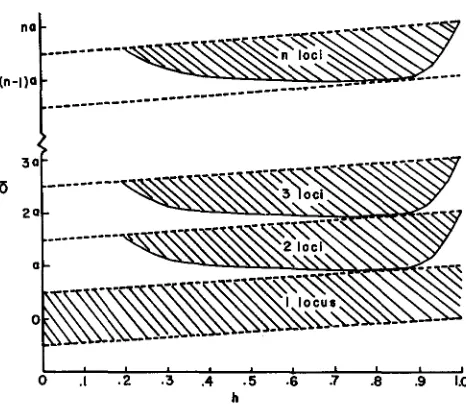
By considerable numerical computation using relations 6a-6c KOJIMA was able to map out the possible stable equilibrium situations for two loci on the assump- tion that the values of a and h are equal for both loci. The result of those compu- tations is shown in Figure 1, modified from KOJIMA’S paper to generalize his results for any number of loci. Along the ordinate are values of the optimum,

0,

scaled in units of a. Along the abscissa are the various values of dominance, h.

The shaded region represents the combinations of

6

and h that will lead to stable intermediate frequencies of q1 and qa such that both loci are segregating. Outside this area there is no stable equilibrium except the trivial ones of one or both loci fixed. We will return to this point later.

SELECTION AND LINKAGE 76

.i

.i

.3 .4 .5 .6 .7 .8 .9 1.0 I h

FIGURE 1 .-A generalization of KOJIMA'S requirements f o r stability of the quadratic optimum mode. The ordinate is the value of the optimum 0 scaled in units of gene effect, a. The abscissa is the dominance h. The shaded areas are the regions of stability for successively larger numbers

of loci. The dashed lines enclose the region of necessary stability.

First, for a fixed value of h, the equilibrium gene frequencies get closer and closer to unity as

O

is increased. At the upper boundary of the shaded region those frequencies reach unity. At the lower boundary the gene frequencies are closer to .50 but do not reach it and are in fact bounded at much higher frequen- cies than one half. For example at h = .8 when the area has its maximum down- ward extension, q = .73 far both loci. Thus equilibrium frequencies are strongly biased toward high values. Second, the shaded region is bounded by a larger region between the two dashed parallel lines, forming a band of width a. This band is a necessary condition on for stability for each value of h. This necessary condition is given by Equations 6a and 6b and simply requires overdominance at each locus at equilibrium. The smaller shaded area gives the necessary and sufficient condition for stability and is smaller because of the extra requirement on

0

imposed by Equation 6c specifying the amount of epistasis between the loci. For the purposes of our present discussion we need only consider the weaker condition given by the parallel dotted lines, since it will be quite strong enough to make the point being aimed at.

that to maintain n loci in a n unfixed state where all loci are of equal additive effect, a, requires that the optimum phenotype fall somewhere between na and (n--3/2)a. That is, the absolute difference between optimum and extreme cannot be greater than 3/2 a. Thus, to maintain, say, ten loci in stable unfixed equilib- rium would require that the optimum phenotype be within 15 percent of the extreme possible for these ten loci.

This may be looked at in another way. Suppose 20 loci each with an additive effect of 3 and a dominance of .5 are segregating. The maximum phenotype due to segregating loci is then 60. If the optimum phenotype is 28, all 20 loci cannot be kept in equilibrium. Loci will be fixed one by one until the maximum effect of segregating loci is less than 30 and this will happen when ten loci are segre- gating. The ten fixed loci will have been fixed half at the plus allele and half at the minus allele so that the mean phenotype is not changed.

The unfixed loci will be maintained in stable equilibrium at gene frequencies very close to unity. However, this is not the only possible stable configuration.

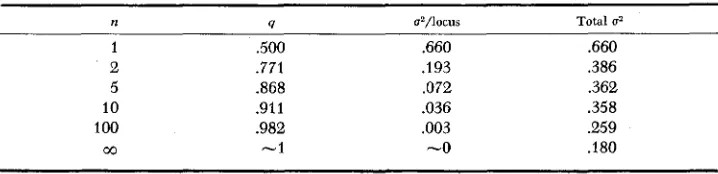
If one of the loci should become fixed by chance at the plus allele, the system decays one step to the next lower stability band. That is because any loci fixed at the plus allele can be regarded as scale shifts in Figure 1 , shifting both the pheno- types and the value of the optimum, but preserving the difference between them. Each time a locus is fixed the remaining loci equilibriate at gene frequencies closer to .50 with the result that each successive random fixation becomes less likely. The number of loci segregating at equilibrium will be a function of recur- rent mutation rates and population size and will increase with an increase in both of these factors (KIMURA and CROW 1964). The fewer loci that are main- tained at equilibrium the farther the gene frequency at each locus is from unity for a given position inside the shaded area. For example with a = 1, h = .8 and optimum one less than the number of loci, two loci can be maintained each at a frequency of .771 while 100 loci will be maintained each at a frequency of .982.

Thus, the more loci maintained at equilibrium, the smaller the genetic variance per locus. The interesting question then arises as to how the total genetic variance on the phenotypic scale changes as the number of identical loci increases. That is, how much genetic variance can be maintained in a population by quadratic opti- mum selection?

TABLE 1

Equilibrium gene frequency and genetic uariance of a character f o r which h = .8, a = I and 0 = (n - I ) when different numbers of genes are segregating

n q az/locus Total o2

1 2

5

10

100 CO

.500 .771 .868 .911 .982 -1

.660 .I93

,072

.036 .003 -0

.660 .386 .362 .358 .259

Table 1 shows the calculations based on equations 1 and

5

of the phenotypic variance maintained at equilibrium for different numbers of loci when a = 1, h = .8 and

6

= ( n - 1 ) .

The table shows that the variance per locus goes down more quickly than the number of loci goes up so that the total variance actually decreases with increas- ing number of loci. This remarkable result then enables us to predict that as more loci concerned with the character are fixed by chance, with fewer and fewer loci segregating at equilibrium, the phenotypic variance for the character will actually increase, reaching a maximum when only a single locus is still segregating with a gene frequency close to .50.

The minimum variance as the number of loci grows indefinitely large is

l f h

l i m V = a 2 ( 1 - h )

n+ CO

where aE is the absolute difference between the optimum for an n-locus system and ( n - 1 ) a . This is a constant irrespective of n since the various bands, as al- ready pointed out, are rigid translations. Thus, for the case we have been con- sidering where h = .8, a = 1 and

o=

( n - 1 ) , the value of E is 0 and

as shown in Table 1. The proof of expression 8 is given in Appendix 11.

When we turn to the maximum variance that can be maintained as the result of a single segregating locus, we can use the usual expression for equilibrium at a single locus

(9)

Substituting ( 3 ) into (9) and using the scale of a, a h and --a for the phenotype we get

_ - _{+ x}

Q = - - + 1

0

-

2 a(l--hz) +2hO 2 (10)

Moreover, the total phenotypic variance from ( 5 ) and ( I O ) is V =

(-

1 -

ex2)

a*

[

1 4- - hz - 2xh (2-xh)

]

2 2

(11)

For x and h of the same sign, which is the only case of interest to us, the maxi- mum value of ( 1 1 ) occurs when the optimum is exactly halfway between the two homozygotes ( x = 0) and the variance is simply

v = -

a? (I+-) h2

2 2

whose maximum value tends to .75 az as h tends to unity. For

-d

= 0 to result

in

a stable equilibrium, h must be less than unity. Thus the maximum variance that can be maintained by genes selected in a quadratic optimum selection system is three quarters of the squared gene effect. This occurs when the optimum is intermediate between the two homozygotes at a single locus and when the degree of dominance is nearly but not quite unity. Without any dominance ( h = 0),

Our conclusion must be, then, that selection based upon the squared deviations from an optimum cannot maintain much variance for a character although i t may maintain large numbers of loci segregating. However, when large numbers of loci are segregating each is maintained so close to fixation that random events are sure to reduce the number of segregating loci to very few where the net selection per locus becomes more substantial.

Stable equilibria are also possible when h

>

1 (overdominance) and for such cases the necessary condition for equilibrium is simply

O >

(n--)a+- 1 ha

2 2

For such overdominant cases the closer the optimum is to its lower limit, given by (13), the closer the equilibrium gene frequencies are to fixation. This is the opposite of the cases of partial dominance where optima close to the lower allow- able limit gave gene frequencies farthest from fixation. The reason is that for overdominant cases, large optima are always closer to the heterozygote than the homozygotes, and always closer to the larger homozygote. However, the larger the optimum the more nearly equal are the relative deviations of the two homo- zygotes and therefore the more nearly alike their fitnesses.

The Effect of Linkage on the Quadratic Model

To test whether linkage makes a substantial difference to the conclusions of the previous section I have examined a number of %locus and 5-locus quadratic deviation cases numerically. The numerical methods are the same as those used in the first paper of this series, that is the method of genetic operators using a digital computer.

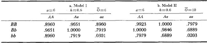
Tables 2a and 2b give the pertinent parameters for two 2-locus models. At the top of each table are given the values of a, h and

6,

the assumption being that the two loci are identical in their action. In the body of each table are given the fitnesses of the nine genotypes calculated from the parameters and from relation

(3) above. For Model I, K = 334.0 and for Model 11, K = 494. The fitnesses are then adjusted to make the maximum fitness unity. These models satisfy the necessary and sufficient conditions for gene frequency equilibrium given in Figure 1. When a = 6 and h = .6, the optimum must lie between 5.5 and 10.8 and Models I and I1 have been chosen to lie just within this interval. These cases

TABLE 2

Parameters and fitnesses for Models I and II

a. Model I - b. Model I1

-

a=6 h=O.6 O=G a=6 h=0.6 0 = 1 0

A A Aa aa A A Aa aa

were chosen to cover extremes of stable gene frequency possible with the quad- ratic optimum model and also different selection intensities. I n neither case are the selection intensities very great at equilibrium since the most frequent geno- types, by far, are the double homozygote AABB and the two single heterozygotes whose fitnesses are nearly the same.

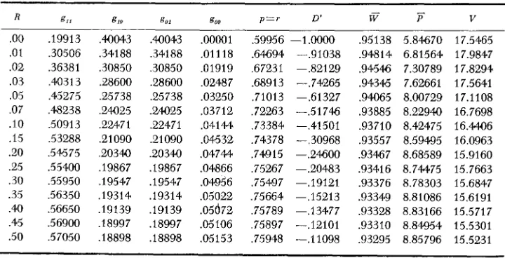
The results for these models are shown in Tables 3 and 4. The tables give the recombination fraction

R,

the four gametic frequencies, the gene frequencies, p , which are the same for both loci, the linkage disequilibrium parameter

D’,

and the mean fitness of the population

w.

D’

is defined in LEWONTIN (1964) as the linkage disequilibrium relative to the maximum possible value, given the gene frequencies. For Model I there are considerable changes in gene frequencies and gametic frequencies with changing recombination, the chief difference appearing between complete linkage ( R = 0) and about 20 percent recombination. The differences in gametic frequencies are quite profound. Linkage increases the repulsion gametes A b and aB until they become 80 percent of the gamete pool at R = 0 while for free recombination they represent only 35 percent of the pool. This corresponds to the magnitude and sign of the relative linkage disequilibrium parameter,

D’,

which is consistently negative indicating a n excess of repulsion linkages. Unlike the heterotic models examined in the first paper of this series

( LEWONTIN 1964) there are no complementary equilibria with an excess of coupling linkages. As will become apparent in the course of this paper, optimum models are characterized b y an excess of repulsion gametes. The second point worth noticing about the linkage disequilibrium is that it exists even at R = .50. This reflects the second characteristics of optimum models, that even when loci are additive on the primary phenotypic scale, very large amounts of epistasis are generated on the fitness scale because fitness is not monotonic with gene dose. The large epistasis results in linkage effects even with free recombination.

TABLE 3

Stable equilibria for Model I , with different amounts of recombination

.oo

.01 .02 .03 .05 .07 .10 .I5 .20 .25 .30 .35 .40 .45 .50 ,19913 ,30506 ,36381 ,40313 ,45275 ,48238 .50913 ,53288 ,54575 .55400 ,55950 ,56350 ,56650 .5 6900 ,57050 .WO43 ,341 88 ,30850 .e8600 ,25738 ,24025 ,22471 ,21090 ,20340 ,19867 ,19547 ,19314 ,19139 ,18997 ,18898 ,40043 .34188 ,30850 .28600 ,25738 .24025 ,22471 .21090 .20340 .I9867 ,19547 .19314 ,191 39 ,18997 ,18898 .00001 .01118 .01919 ,02487 ,03250 .03712 .04144 ,04632 ,04744 .04866 .04956 ,05022 ,05672 .05106 ,05153

,59956 -1.0000 .64694 --.91038 ,67231 -.82129 .68913 -.74265 ,71013 -.61327 ,72263 -.51746 ,73384 -.41501 ,74378 --.30968 ,74915 -.24600 .75267 -.20483

,75664 -.I5213 ,75789 -.I3477 ,75497 -.19121

,75897 -.I2101 ,75948 -.11098

The third important and interesting effect of linkage is shown in the last three columns of Table 3 . As for heterotic models, the effect of tightening the linkage is to increase the mean fitness,

v,

of the population. This increase is small how- ever, about 2 percent, although in terms of genetic load it represents a decrease of 26 percent. It is the composition of the mean fitness that changes in an inter- esting way. Expression

(4)

shows that the loss of fitness is due to two components: the squared deviation of the population mean phenotype from the optimum,

(S-0) 2; and the deviations of individuals from the population mean represented

by the phenotypic variance, V . As the last two columns of Table 3 show linkage has two opposite effects of fitness. The tighter the linkage, the closer the popula- tion mean to the optimum, 6. This has the effect of making fitness higher for close linkage. However, the tighter the linkage, the greater the within population variance (with the exception of R = 0) and this has the effect of lowering the population fitness. The net effect of the two is a slight increase in fitness with increasing tightness of the linkage.

Table

4,

giving the results for Model I1 shows results that are in all respects parallel to those of Model I except that the differences are very much smaller.

D',

however, is about as large in Model

I1

as in Model I although the absolute linkage disequilibrium is less. This shows that even when selective differences are small, optimum models generate epistatic deviations that are large in comparison to additive deviations so that relatively severe linkage disequilibria result.

The third quadratic optimum model to be considered is a 5-locus model in which the assumptions are the same as for the 2-locus models. We assume five identical loci determining phenotype additively between loci. The additive effect, a = 6, the dominance h = .8 and the optimum, = 24. This satisfies the require- ments for stable equilibria given in Figure 1, since the optimum falls in the shaded region. It is, as a matter of fact, the extension of the two locus case with a = 6, h = .8 and

0

= 6 discussed earlier. that is,

0

= (n-1 )

.

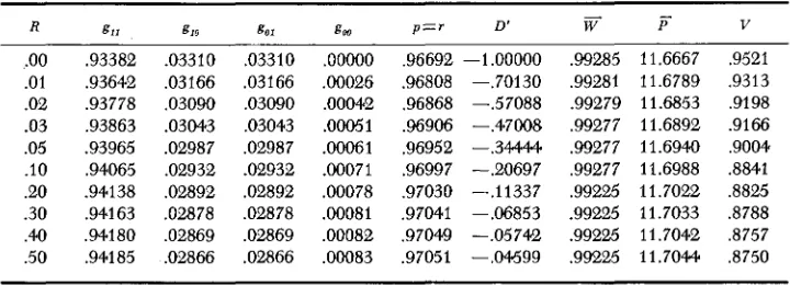
Table 5 shows the fitnesses of the different genotypes based upon these parameters. Because all loci are identical only the number of loci homozygous 00, heterozygous 01 and

- -

TABLE 4

Stable equilibria for Model I I with different amounts of recombination

R

.oo

.01 .02 .03 .05 .IO .20 .30 .40 .50 g11 .93382 .93642 .93778 ,93863 .93965 ,94065 .94138 .94163 ,94180 .94185 g10 .03310 ,03166 ,03090 .03043 .02987 .02932 .OB92 ,02878 .02869 .02866 go1 .03310 ,03166 ,03090 ,03043 .02987 .02932 ,02892 .02878 ,02869 .OB66 g, .ooooo ,00026 ,00042 .00051 .00061 .WO71 .WO78 .WO81 .00082 .OOO83

p = r D'

.96692 -1 .OOOOO

.96808 -.70130 .96868 --.57088 .96906 --.47008 .96952 --.34444 .96997 -.20697 .97030 -.I1337 ,97041 --.Of3853 ,97049 -.05742 .97051 --.04599

TABLE 5

Fitnesses for Model Ill. All loci are identical and for each a = 6, h = .8 and 6 = 24 Number of loci with genotype

1/1 1 /o

0 0

0 1

0 2

0 3

0 4

0 5

1 0

1 1

1 2

1 3

1 4

2 0

2 1

2 2

2 3

3 0

3 1

3 2

4 0 4 1

5 0

o i n Fitness

5 ,98800

4 .99232

3 ,99568

2 .99808

1 ,99952

0 1

.ooooo

4 ,98800

3 .98272

2 .97648

1 ,96928

0 .96112

3 .89200

2 ,87712

1 36128

0 ,84448

2 .70000

1 ,67552

0 ,65008

1 ,41200

0 ,37792

0 .02%00

homozygous 00, but not the identity of the loci, need be considered. A homozy- gote 00 then has a phenotype of 6, a heterozygote 01 a score of 4.8 and a homo- zygote 11 a score of -6.

Table 6 is a sample of the results of this model showing equilibrium gametic frequencies, gene frequencies, linkage disequilibruium parameters, variances, and mean fitnesses for selected recombination values. The gametes are given in their binary form, 00000 being a gamete with all five loci represented by the allele with a positive effect on the phenotype and 11 11 1 stands for a gamete with all five loci represented by the allele with a negative effect on the phenotype. Only the gametes with reasonably high frequencies are given in Table 7 and it will be noticed that these are the 16 gametic types with a majority of 0 alleles. Gametes with three or more I alleles never exceed a frequency of .OO172, at the loosest linkage shown and they all decrease to zero at the tightest linkage. The linkage disequilibrium parameters in the table represent all possible situations, given the fact that the chromosome is left-right symmetrical. Thus,

DI2

= D’,5 and DI3 = D’,,, etc. The same symmetry applies to gene q1 q5, q3 = q3. The last column gives the results to be expected if all the loci were at linkage equilibrium, although even a recombination fraction of .50 departs slightly from such an equilibrium situation.

Y

d

N

2

3

3

3 ?

3

3

2 ?

0

?

10

3

?

2

?

3

3

?

Y)

B

B

SELECTION AND LINKAGE

TABLE 7

Fitnesses for Models IV, V and VI. See text for methods of determining t h s e fitnesses

Number of loci with genotype Fitnesses

1 / 1 o/1 o/o Model IV Model V Model VI

0 0 5 0.0 ,0679 .i754

0 1 4 0.0 ,1105 ,2670

0 2 3 0.0 .I612 .3693

0 3 2 0.0 ,2114 .4654

0 4 1 1

.o

.2487 .5342

0 5 0 1

.o

,2624 .5594

1 0 4 0.0 .I612 .3693

1 1 3 0.0 ,2114 ,4654

1 2 2 1

.o

,2487 5342

1 3 1 1.0 .2624 ,5594

1 4 0 1

.o

,2487 5342

2 0 3 1

.o

.2487 .5342

2 1 2 1

.o

,2624 5594

2 2 1 1

.o

,2487 ,5342

2 3 0 0.0 .2114 . 6 5 4

3 0 2 1

.o

,2487 ,5342

3 1 1 0.0 .2114 ,4654

3 2 0 0.0 ,1612 .3693

4 0 1 0.0 ,1612 .3693

4 1 0 0.0 .I 105 ,2670

5 0 0 0.0 ,0679 .1754

K -c 1.0 k l . 0 zk 2.3

H2 1

.o

0.2 0.2

effect is extremely small since the population at equilibrium is very close to perfect fitness for all recombination values. As in the previous cases, tight linkage brings the population mean closer to the optimum which accounts in part for the increase in fitness. The changes in gametic and gene frequencies are also reflected strongly in the changes in phenotypic variance. As for the 2-locus models, the phenotypic variance increases steadily with tightening of linkage except for com- plete linkage where all extreme gametic types are completely absent with a con- comitant loss of phenotypic variance. The general increase in phenotypic variance with tighter linkage is in part due to the changing of gene frequencies toward more intermediate values.

The general picture that emerges from treating 5-locus cases such as Model I11

is that all effects of linkage are the same as in cases of fewer loci but the magni- tude of the effects is smaller. This dilution of effects with increasing numbers of loci in the quadratic optimum model is caused by the much higher equilibrium fitness possible with many loci. I n addition the gene frequencies at each locus are much closer to fixation at equilibrium and the genetic variance per locus is much smaller as shown in Table 1. Thus, the amount of phenotypic variance that can

crease this variance. Thus, tight linkage increases the equilibrium phenotypic variance for the 2-locus case by a maximum of 16 percent over the free recombi- nation case, while for the 5-locus model this increase is 24 percent. This variance and the intermediate gene frequencies are maintained at a relatively low level of genetic load.

Double Truncation Models

I n the first part of this paper

I

have shown that truly stable equilibria are difficult to maintain with large numbers of loci with a quadratic deviations model. Moreover, the amount of genetic variance maintained at these equilibria is not great. ROBERTSON (1956) has shown that some other types of optimum model are even worse in this respect in that they predict no stable intermediate equi- libria. While linkage does increase the variance maintained at equilibrium in the quadratic deviations model, it does not change the situation materially. It would seem, then, that selection for an intermediate optimum is not likely to account for very much genetic variation in populations. This is not the case however. In this section I will examine the rate of approach to fixation of gems for optimum models that do not lead to true stable equilibria. As it will turn out linkage may cause the retention of large amounts of potential genetic variability for extremely long periods although not forever.

The models used to investigate this problem are of the following nature. Five loci determine the genetic score, the loci being all identical in effect, the effects at the various loci adding to each other (no epistasis). At each locus the three genotypes 11, 01 and 00 have the effects a, a h and -a on the phenotypic score. The actual phenotype corresponding to any genotype is assumed to be normally distributed with a mean equal to the genetic score and a variance arising from environmental differences and segregation of genes at other loci than those under investigation. Selection operates by rejecting completely all individuals falling outside the limits K a and allowing as parents of the next generation all indi- viduals inside these limits. Because each genotype has a normal distribution of phenotypes around its genotypic mean, it is easy with a table of the normal distribution to find the probability that an individual of a given genotype will fall inside the limits i: Ka. This probability is, by definition, the fitness or adap-

tive value of the genotype. If all genotypes have the same environmental variance then clearly the closer the genotypic mean is to zero, the center of the acceptance region, the greater the fitness. When genotypes have different variance, however, the situation may be more complex. These relationships are shown in Figure 2. The first three double truncation models to be considered are those given in Table 7 as Models, IV, V and VI.

For each model the table gives the truncation limits, K , the initial heritability, H 2 , and the resultant fitnesses of each genotype. In all three models the popula- tion is started in linkage equilibrium with gene frequencies .55, .60, .65, .70 and .75 for the five loci in order on the chromosome. This gives an initial genetic variance uQ2 = 2.225. The environmental variance around each genotypic mean

2.225

(1-H2)

H2

FIGURE 2.-Diagrammatic illustration of double truncation selection. Each normal distribu- tion shown has a mean, ui, given by the genotype and a variance caused by environmenta1 variations. All individuals falling between the heavy vertical lines survive while those outside this region do not. The shaded area is the fitness of a genotype.

For Models IV, V and VI H z is assumed the same for all genotypes. In Model IV it is 1.0 so that each genotype is either lethal, if it falls outside the limits +- K , or

perfectly fit if it falls within these limits. Model V has the same selection limits but H z = .20 so that 80 percent of the variation is environmental. Model VI de- creases the stringency of selection by widening the limits to K = 2.3, while hold- ing heritability at 20 percent.

The changes in population structure during the course of selection are shown in Figures 3,4 and 5. Part A of each figure shows the changes in gene frequencies with time. Part B shows how mean fitness changes and Part C how linkage disequilibrium behaves. To avoid confusion only cases of tight ( R = .01) inter- mediate ( R = .05) and loose ( R = .235) linkage are given for Parts A and C. As usual these are the linkage values between adjacent genes so that the linkage between outside markers is considerable weaker.

The results shown in Figure 3 are typical of the three cases but the results are more drastic because of the drastic selection differential. At first there is a sharp change in gene frequencies at all loci to bring the mean phenotype of the popula- tion close to zero, the center of the acceptable range of phenotypes. This, in turn accounts for the rapid rise in fitness shown in Figure 3B. This process occupies only about two generations and there is no differentiation between cases of loose or tight linkage. After this point, however, the fate of loosely linked and tightly linked genes is very different. Loosely linked genes go to fixation in a symmetrical fashion with one locus temporarily stalled near q = .50. After about 90 genera- tions only this locus is still segregating to any marked degree. As the other four loci get arbitrarily close to fixation, the fifth locus will have virtually no selection pressure on it since the heterozygote and two homozygotes at this locus have a

.9

li)

.a

1

IO 2 0 10 *O 8 0 60 10 80 90

GENERATION

C.

-.a I I I ,

I O 20 10 4 0 6 0 1 0 8 0 90

G E N E R A T I & '

773

gene frequencies after becoming symmetrical around .50 remain essentially unchanged for 90 generations. The most deviant gene frequencies at 90 genera- tions are ql = .675 and q5 = .336, for R .01. With R = .05 the three intermedi- ate gene frequencies, q2, q3 and q, actually conuerge toward .50 as generations pass, although this is temporary. The rapid increase in fitness has occurred through the fixation of gametic types so that there is a marked deficiency of coupling gametes. This is seen in Figure 3C showing all coefficients of linkage disequilibrium as negative.

One very interesting feature of Figure 3B is the change in the order of mean fitnesses with time. In early generations the tighter the linkage the higher the mean fitness. However, as time goes on the more loosely linked situations slowly increase in fitness passing the more tightly linked case above them. By generation 90 the most loosely linked case is more fit than all except the most tightly linked case, and the next most loosely linked case is beginning its period of more rapid rise. This turnover process eventually results in a complete reversal of the order of fitnesses although this is of very little significance since all cases are very near their maximum possible fitness at that point. As for the quadratic deviations models. loss of mean fitness of the population arises from two causes: deviation of the population mean from the center of the acceptable zone, and phenotypic variance within the population causing individuals to fall outside the acceptance zone. In the case of Model IV all this variance is genetic since the heritability is 1.0, but for Models V and VI some of the variance is nongenetic. Figure 3B

can then be used as a n index to the genetic variance in later generations. In the first two generations the rapid increase in fitness is due to reducing the deviation of the population mean from the middle of the acceptance range and this is the same for all degrees of linkage. Following that increase, the changes in popula- tion fitness are the result of the loss of genetic variance, the highest fitness cor- responding to the lowest genetic variance. We see that in the tightly linked case there is extremely rapid loss of genetic variance by the process of elimination of coupling gametes; while for loose linkage the loss of variance is slower and occurs by fixation of genes. Thus, the relative amounts of genetic variance undergo the same changes in order as do the fitnesses in Figure 3B. Despite the very low genetic variance in the tightly linked cases, the opportunity for the manifestation of new genotypes is much greater because gene frequencies are held at inter- mediate frequencies. The tightly linked genes then have a greater potential to respond to new selective forces because potential genetic variability is maintained in the form of linked complexes.

R . C . LEWONTIN 774

I

A. I

O J I

J

40 SO 6 0 7 0 8 0 so

I O 2 0 ao . _

G E NE RATION

-

W

.LLB

.t SO

IO 2 0 a o 40 BO 60 T O 8 0 90

GENERATION

0

IO 2 0 3 0 40 5 0 eo TO 8 0 9 0

G EN E R AT I ON

775

A

1 I

S I O I8 2 0 25 3 0 38 4 0 a 8 0

G E N E RAT1 ON

.ss

.!I 0 ii

8 I O I S LO 2 6 10 3s 4 0 4 8 so

GENE R A l l ON

0

-.1

D'

-.4

-.t C

S I O I 5 2 0 25 3 0 38 4 0 4 8 so G E N E R A T 1 ON

776

Homeostatic Models

The last models to be discussed are the same as Models IV, V and VI except that the assumption of equal environmental variance no longer holds. Models VI1 and VI11 whose fitnesses are given in Table 9, are based on LERNER'S

hypothesis that the greater the degree of heterozygosity, the smaller the environ- mental sensitivity of a metric trait. I n particular Model VI1 is based upon setting the environmental variances of the genotypes progressively greater for lower

TABLE 8

Environmental variances (uez) and initial heritabilities in relation to initial genetic variances ( 0 ~ 2 ) for different genotypes in Models V I 1 and VlII

Number of loci heterozygous

5 4 3 2 1 0

1.000 0.0 1.000 0.0 .833 0.2 .500 1

.o

.667 0.5 ,333 2.0

.500 1

.o

.250 3.0

.333 2.0 ,200 4.0

.I67 5.0 .I67 5.0

TABLE 9

Fitnesses for Models VI1 and V I I I . See text for method of determining fitness

Number of loci with genotype

1/1 1 / 0 o/o Model VI1 Model VI11

Fitnesses 0 0 0 0 0 0 1 1 1 1 1 2 2 2 2 3 3 3 4 4 5 0 1 2 3 4 5 0 1 2 3 4 0 1 2 3 0 1 2 0 1 0 5 4 3 2 1 0 4 3 2 1 0 3 2 1 0 2 1 0 1 0 0 .0789 ,0686 ,0861 .1685 .4986 1

.oooo

,1595 . 2 a 2 .4102 ,3294 ,4986 .225 1 .36% ,4102 .I 685 ,2251 .2402 ,0861 .1595 ,0686 .0789 ,0789 .1103 .I 585 . 2 a 2 .4102 1 .0000

.I 595 .2113 .2809 .36% .4102 .2251 .2634 .b09

degrees of heterozygosity. The initial heritabilities and environmental variances for the two models are given in Table 8. The result of the changing heritability is that the pentuple heterozygote is more fit than any other genotype (Table 9) and this, in turn, results in a stable equilibrium of gene frequencies at p q = .50

for all loci.

Tables 10 and 11 give the stable equilibrium results for various values of re- combination. Only 16 gametic types are shown, but their 16 reciprocal types have identical frequencies. What is particularly noteworthy i n these results is the appearance of alternating coupling and repulsion linkages for tighter linkages ( R = .065-.070). All other optimum models described in this paper gave only repulsion linkages. The coupling linkages which appear in Models VI1 and VI11

represent the stable configuration for these models and cause a maximization of fitness. Solutions also exist when all linkage are repulsion type but these are

unstable and result in fitness minima.

I have not given the picture of the early stages of selection for Models VI1 and

VI11 since they give stable equilibrium, but these early stages have been computed

and a single example is given in Figure 6. Starting in linkage equilibrium, the populations at first produce all repulsion linkages, but as the gene frequencies

TABLE 10

Results of Model VII. Symbols are as explained in the text

~ ~ ~~

~~

R between adjacent loci

Gametes ,045 ,050 ,060 .07 .os .10 .14 2 3 4

00000 00001 00010 0001 1 00100 00101 00110 001 11 01 000 01001 01010 0101 1 01 100 01 101 01110 01111

D’ 12 D’ 13 D’ 14

D 15 D’ 23 D’ 24

W

-

.00016 .00205 ,00861 .00328 ,00999 .06109 ,01276 ,00328 ,00861 ,04706 ,20724 .01109 ,01276 .04706 ,01290 .00205 ,00034 ,00351 ,01091 ,00556 ,01245 .06138 ,01804 ,00556 ,01091 .05164 .I6610 .06138 ,01804 .05164 .01905 .00351 .00105 ,00829 .01474 ,01144 .01413 .MO46

,0296 7 .01144 ,01474 .05890 .lo172 .05046 ,02967 .05890 ,03612 ,00829 ,00179 .01144 .01682 .01525 ,01537 .MO9 ,03440 .01525 .01686 ,05774 ,07948 ,04509 ,03440 .05774 ,04188 ,01144 ,00249 .01328 .01840 .01795 .01716 .04352 .03615 .01795 ,01840 .(I5481 .07041 ,04352 .03615 .05481 .04198

. 0 1 328

.00388 .01562 .02000 .02322 .01948 .04261 ,03749 ,02322 .02000 .04959 ,05943 ,04261 ,03749 .04959 ,04016 ,01562 ,00666 ,01930 ,02324 .02765 .02346 .OW31 .03725 .02765 ,02324 .04380 .04933 ,04031 ,03725 ,04380 ,03745 ,01930 ,01085 ,02351 .02590 ,03123 ,02623 ,03796 .03550 .03123 ,02590 ,03904 .04147 ,03796 ,03550 ,03904 ,03516 ,02351

-.59512 -.52904 --.43516 -.37836 -.33236 -.25792 -.17792 -.11036 +.35244 $.24136 f.14528 -.02228 - . W O O -.06264 -.06588 -.05652 -.24484 -.1604.0 --.05548 -.03840 --.03752 -.04700 --.04876 -.04784 +.09212 +.OW80 --.03264 -.03616 -.03652 -.04832 -.04.844 -.05400 --.64448 --.54976 -.32604 -23696 -20656 ---.17768 -.I4140 -.I0120 f.42628 t.31088 +.08208 f.00636 --.01848 -.04236 -.05548 -.05332

R.

TABLE 11

Results of Model VIII. Symbols are as ezplained in the text

R between adjacent loci

Gametes .005 .01 ,065 .07 .08 .io .14 ,034

00000

00001 00010

0001 1

00100 00101 001 10 001 11 01000 01001 01010 01011 01100

01 101 01110 01111 D’ 12 D 13 D 14 D’ 15 D 23 D 24 W

-

.ooooo

.00000 .00003 .00000 .00003 .00457 .00003 .00000 .00003 .00436 ,48197 “7 .00003 ,00436 .00003 .00000 .00000

.ooooo

.om12 .Ooooo .om12 ,00921 .00014

.ooooo

.00012 .00879 .46321 .00921 ,00014 .00879 ,00013

.ooooo

.00208 .00892 ,01686 .01159 .01585 .04915 ,02778 .Oil59 .01686 .05649

.1 0992 . M I 5 ,02278 ,05649 ,03057 ,00892 .00334 .01241 .01909 ,01555 .01743 . w 7 9 ,03253 ,01555 .01909 ,05527 .08301 .04479 ,03253 .05527 ,03693 .01241 ,00508 ,01555 .02133 .01960 02003 .04222 .03523 .01960 .02133 ,05112 ,06627 .04222 .03523 .05112 .03850 .01555 .00767 .01865 .ow22 .02504 .02295 .om0 .(I3642 .02504 .02322 .b635 .05372 . W 6 0 ,03642 .04535 .03713 .01865

.01206 ,0226 1

.02618 ,02883 .02655 .03794 .03565 ,02883 .02618 .03993 . W O .03794 ,03565 .03993 .03512 ,02261 .01713 .02628 .02809 .03125 .0b38 .03565 .03402 .03125 .0b09 .03622 .03782 .03565 .03402 .03622 .03365 .02628 --.98136 -.96160 --.42476 -.35720 -28544. -.20172 -.12544 -.07180 +.96380 +.92580 +.08748 +.01024 --.02966 -.05016 -.04912 -.03788 +.92860 +.85592 --.00924 -.02420 --.02800 -.03712 -.I3448 -.03520 $.96468 +.92756 +.09828 +.02044 --.01828 -.OM20 --.OM4 -.03672

.59257 .57275 ,34583 ,33754 .33158 .32637 .32058 .31612 --.94652 --.89128 -.06548 -.03944. --.03324 -.03928 -.03660 -.03204 --.98220 -96324 -.34716 -.24988 --.19212 -A5152 --.lo804 -.06832

reach equilibrium, some of these repulsion linkages disappear and are replaced by coupling phase linkages. The particular linkages shown in Table 10 are not the only possible equilibria. There are ten alternative configurations in which the majority of gametic types form a pair of the type 11100/00011 or 10110/01001, or, etc. All these equilibria have the same mean fitness. As Table 10 shows there are very considerable linkage disequilibria between adjacent genes even when these recombine as much as 6 percent. When adjacent recombination fractions are 1 percent, the outside markers, which are then

4

map units apart, are in very great disequilibrium (D’ = .84 for Model VIII).

The most remarkable feature of these models is the very large increase in fit- ness that results from linkage. In Model 8, if the adjacent genes recombine 1 percent the average equilibrium fitness is .57275 compared with fitness of .3161Q when

R

= .24. This is an increase of 81 percent in fitness and if the genes are really tightly linked ( R = .OOl) fitness is essentially doubled.

t

General Implications of the Results

S E L E C T I O N A N D L I N K A G E

D'

-.3

-

-.4 .

-.SI I

G E N ER AT1 ON

FIGURE 6.-Li&age disequilibrium parameters, D', (ordinate) at various times (abscissa)

5 I O 15 2 0 2 5 3 0 35 4 0 4 5

f o r Model VI11 with R = ,001.

mal genetic strategy. On the other hand, in environments undergoing rapid fre- quent fluctuation, a less labile system is optimal and tight linkage is at a dis- advantage.

The other point of general interest is the degree to which populations may be permanently out of linkage equilibrium. In the earlier papers on this subject

KOJIMA and I have pointed out that interaction between loci in determining fit-

ness is necessary if any permanent linkage disequilibrium is to result. By inter- action we have meant departures from additivity between loci and this follows from our particular model of natural selection in discrete generations. When a continuous generation model is used, the definition of interaction is the deviation from multiplicatiueness between loci, or additivity on a logarithmic fitness scale

(KIMURA

1956). Thus, whether or not a particular scheme of fitnesses leads to linkage disequilibrium depends in part on the model of the breeding structure. For optimizing models, however, interaction is present irrespective of the dis- creteness of generations because the fitnesses do not bear a simple relationship to the rest of the phenotype. On either discrete or continuous generation models, optimizing selection results in very large amounts of interaction on the fitness scale and this, in turn, results in linkage disequilibrium for even the loosest link- ages. To the extent that genes are selected to produce optimum intermediate phenotypes, and this must be a common mode of selection, to that extent linkages play a n important role in the genetic change in the population and linked com- plexes of genes, out of equilibrium, should be found in natural populations.

Over the past eight years I have had many occasions to discuss these matters with DR. KEN- ICHI KOJIMA and I am deeply grateful for the illuminating insights he has given me.

S U M M A R Y

This paper is concerned with the genetic structure of populations subject to “optimizing” selection, that is, selection favoring some intermediate phenotype and discriminating against phenotypes at both extremes. A number of specific models have been examined in which the fitness of phenotypes falls off with increasing deviation from the optimum phenotype. For freely recombining genes virtually no optimum model leads to a maintenance of significant amounts of genetic variation in a permanently stable state. An exception to this rule is a model in which multiple heterozygotes have a lower environmental sensitivity than other genotypes. When recombination is restricted, however, long-time quasi-stable equilibrium of gene frequencies result. The rate of increase of fitness with time before the quasi-stable equilibrium is reached is also strongly affected by linkage with tight linkage causing rapid initial increases in fitness but lower rates of increase in later generations.

APPENDIX I. Proof that shaded area

in

Figure 1 represents the necessary condition for stable equilibrium of n loci.

Let

O

= optimum. Pj = mean genotypic value due to jth locus.

P

= mean genotypic value. a = additive effect per locus. h = dominance effect per locus. Then KOJIMA (1959) shows that a necessary condition for stability is that for all

i

a ( h i - 1 ) 2

<

6

<

P-Pj

+

- a ( h - I )

2 P-Pj

+

Now ( 1 ) specifies the following three properties: (a)

0

lies in an interval whose width is a ; (b) The upper and lower limits of

6

are each linear in h with slope a/2; (c) Lower limit of

O

= P-Pj when h = 1. W e thus have a band of the shape and slope shown in Figure 1 for each locus relating the dominance h to the optimum

0.

Since we are looking f o r a necessary condition we want the simultaneous condition on all the

i

loci which is as broad as possible. But this will be given by the intersection of all the conditions and will be as broad as possible when all bands are identical and include the same region of the h, 6 p l a n e since they are all of fixed width a and fixed slope h/2. This will occur when

for all

i

and i.

-

( 2 ) F-P, = P-P,

Since

p

=

f:

Pi, if ( 2 ) is true then

3 = 1

-

( 3 )

(3) and condition c above

(4)

Conditions a, b and c in conjunction with (4) are the required area.

P-Pi = nPj-Pj = (n-1)Pj

.

Finally, when h = 1 , Pi = a because of fixation of the plus allele. Thus, from

6

= ( n - l ) a when h = 1 .

APPENDIX 11. Derivation of limiting phenotypic variance maintained by the quadratic optimum model

a(h2-1) (1-2qi)

+

2[1

+

h ( l - Q j ) ] [p-Pj--O-l = 0

Expression 7a of the text states that at equilibrium ( 1 )

for all i.

maximize the variance, ( 1 ) becomes, for n loci

( 2 ) a(h2-1) (1-2q)

+

2 [ 1

+

h ( l - 2 q ) ] [ ( n - l ) P j -

d ]

= 0

Setting q = 1 E and ignoring higher p w e r s of E ,

( 3

1

Pi = aq2

+

2pq ah--p2a = a [ 1 - 2 ~ ( l - h ) ]

so that from ( 2 ) and ( 3 )

(4) a ( h 2 - 1 ) ( 2 ~ - 1 ) + 2 [ 1 +h(2~-1)][(n-l)a-6--2~(1-h)(n-I)a] = O I t was proved in Appendix I that (n-I ) a -

6

is a small constant for all values of n. Therefore, as tz grows large without bound the left hand side of (4) will

also grow without bound unless n e is bounded.

782

Therefore

h E = O

n+ m

(5)

Setting

0

- (n- 1 ) a = aE and rearranging ( 4 ) yields

( l f h ) -2E 4(1 -h ) lm ne =

1'

n+ m

Finally, the variance at a single locus is (from text equation

5 )

( 8 ) Ujz 2a2(1-h)'E

ignoring higher powers of E . Therefore the limiting variance of total phenotype

from ( 7 ) and (8) is

LITERATURE CITED

BODMER, W. F., and P. A. PARSONS, 1962

FISHER, R. A., 1950

KIMURA, M., 1956 A model of a genetic system which leads to closer linkage by natural selec-

KIMURA, M., and J. F. CROW, 1964 The number of alleles that can be maintained in a finite population. Genetics 49: 725-738.

KOJIMA, K., 1959a Role of epistasis and overdominance i n stability of equilibria with selection. Proc. Natl. Acad. Sci. US. 45: 984-989. - 1959b Stable equilibria for the optimum model. Proc. Natl. Acad. Sci. U.S. 45: 989-993.

A comparison of purebred and crossbred selection schemes with two populations of Drosophila pseudoobscura. Genetics 48: 57-72.

Linkage and recombination i n evolution. Advan. Genet. 11: 1-100.

The Genetical Theory of Natural Selection. Clarendon Press, Oxford.

tion. Evolution 10: 278-287.

KOJIMA, K., and T. KELLEHER, 1963

LERNER, I. M., 1954 Genetic Homeostasis. Wiley, New York. LEWONTIN, R. C., 1964

LEWONTIN, R. C., and K. KOJIMA, 1960

MATHER, K., 1941

ROBERTSON, A., 1956 The effect of selection against extreme deviants based on deviation or

WRIGHT, S., 1935 Evolution in populations in approximate equilibrium. J. Genet. 30: 257-266. The interaction of selection and linkage. I. General considerations;

The evolutionary dynamics of complex polymorphisms. heterotic models. Genetics 49: 49-67.

Evolution 14: 468-472.

Variation and selection of polygenic characters. J. Genet. 41: 159-193.