ANALYSIS OF COMPLEX ALLOZYME POLYMORPHISMS IN A BARLEY POPULATION

IN A BARLEY POPULATION1 B. S . WEIR2, R. W. ALLARD3 AND A. L. KAHLER3

University of California, Davis, California 95616 Manuscript received December 27, 1971

Revised copy received June 26, 1972

ABSTRACT

Genotypes of 68,230 individuals taken from 10 generations (F,-F,, F,,-F,,, F24-F26) of an experimental population of barley were determined for four

esterase loci. The results show that frequencies of gametic ditypes changed significantly over generations and that striking gametic phase disequilibrium developed within a few generations for each of the six painvise combinations of loci which were monitored. The complex behavior of these four enzyme loci in the population is attributed to interactions between selection and restriction of recombination resulting from the effects of linkage and/or inbreeding.

HIS is the third in a series of papers dealing with the analysis of the fre-

T

quency of allozymes at four esterase loci in Composite cross

v

(CCV), an experimental population of barley (Hordeum uulgare L.) developed from inter- crosses among 30 barley varieties from various parts of the world. The first paper (KAHLER and ALLARD 1970, referred to below as

I)

described the electrophoretic techniques used to detect the allozymes and presented the results of formal ge- netic studies of these esterase loci. In the second paper (ALLARD, KAHLER and

WEIR

1972, referred to below as II), the history of CCV was described and the single-locus frequency data were analyzed. The results showed that mutation, migration, and genetic drift had at most trivial effects and that selection and mat- ing system were the major forces responsible for the patterns of genetic change which occurred in the population. In this paper we extend the analysis of data for CCV to pairs of loci. It will be shown that interactions between selection and restriction of recombination due to linkage and/or inbreeding play a predominant role in the behavior of these four enzyme loci in the population.

TWO LOCUS DATA

The materials on which this study was conducted and the methods employed in obtaining the data are described in detail in I and I1 and hence will not be pre- sented here. The basic data consisted of the multilocus esterase genotypes of

Supported in part by grants from the National Institutes of Health (GM-10476) and the National Science Foundation

Department of Agronomy and Range Science. Present address: Department of Mathematics, Massey University,

(GB-13213).

Palmerston North, New Zealand.

a Department of Genetics.

506 B. S. W E I R , R. W. ALLARD AND A. L. K A H L E R

68,230 individuals from 10 generations of CCV: three early generations (F4, F,, F,)

,

four intermediate generations (F14) F,,, F16, FIT) and three late generations

(FZ4,

F,,,

F2,). The four loci monitored, EA, EB, EC and ED, here designated A, B, C and D, are represented by four, three, three and four alleles, respectively, in CCV (I, 11). Thus, considering each locus individually, there are 6 genotypes for Loci

B

and C and 10 for Loci A and D; considering the loci pairwise there are 36 genotypes for the B-C combination, 60 for the A-B, A-C, B-D and C-D combina- tions, and 100 for the A-D combination. A few of these genotypes cannot be dis- tinguished phenotypically due to recessiveness of a null allele at the D locus, o r to specific interactions between the A2 and B2.7 alleles (I, 11). Nevertheless. the number of genotypes that can be identified is large and, hence, for ease of presen- tation we seek to reduce these numbers in some way. There is another reason for such reduction. CCV practices 99.43% self fertilization (11) so that certain heterozygotes (especially double heterozygotes representing rare alleles) are infrequent in the population and such heterozygotes are sometimes not present even in the large samples studied. This causes problems in analyses which attempt to take all genotypes into account, We use the two following methods of reducing and simplifying the data: (1) consider homozygous classes only, thus reducing the number of genotypes from 36 to 9 for the B-C combination, from 60 to 12 for A-B, A-C, B-D and C-D combinations, and from 100 to 16 for the A-D combination; (2) combine the data into two allelic classes per locus, one consisting of the most frequent allele and the other consisting of all other alleles combined.

ANALYSIS O F HOMOZYGOUS CLASSES

The data for the six possible painvise comparisons of homozygotes in each of 10 generations of CCV are too extensive to be given in their entirety. However results are similar within comparisons between pairs of the three tightly-linked loci A,

B

and

C (B

+ 0.0023

*

0.0007 -+ A + 0.0048 f 0.0008 9 C), within

comparisons of each of these loci with the non-linked locus D, and also within the early, intermediate and late generations. Consequently data will be given for only one early, one intermediate and one late generation for one pair of linked loci and one pair of unlinked loci, since these partial data suffice to bring out the main features.

TABLE 1

Relative deviations [(observed two-locus numbers minus the product of one-locus numbers/N) x lOOO] for loci B and D in generations 6,17, and 26 of CCV

Locus D+

Locus Bt 11 22 33 44.

Generation 6 N = 1006 x2 = 5.1 (NS) Generation 17

N = 2461

x 2 = 49.5

Generation 26

N = 3083

x2 = 2443.8

11 22

33

11 22

33

11 22

33

- 5 + 4 + I

+ 8

+ 3

+4fJ

-48 - 1 -12

- 1 $ 6 + I

+ 2 - 5 - 1

+ 2 - 8 - 1

- 2 + 7 + 8

+ I + 2 - 7

- 9 -25 -1 0

+

9 4-20 +I4

- 1 - 1 - 1

- 1 + 3 - 4

+

The allelic designations for locus B are B1.6 = 1, B2.7 = 2, B 3 . 9 = 3 and for locus D they are

D6.4 = 1, D6.5 = 2, D6.6 _{3 and DN} = _4.

favorably and that others (e.g.

B2.'

and

D6..")

interact unfavorably with each other in their homozygous combinations. By generation 26 departures have be- come very large. Inspection of this table shows that each of the four alleles a t the

D

locus interacts favorably in at least one of its homozygous combinations with the three alleles at the

B

locus, and unfavorably in at least one combination.

Re-

sults are closely similar for the two other comparisons of unlinked loci (A-D and Table 2 gives results for the tightly-linked pair of loci. B and C. In this case departures from expected values are significant by generation 6 and it can be

C-D)

.

TABLE 2

Relative deviations [(observed two-locus numbers minus the product of one-locus numbers/N) x 100OJ for loci B and C in generations 6,17, and 26 of CCV

Locus B+ 11 22 33

Generation 6 11

+

17 - 5

-

11

N = IO06 22 - 28 + I

+

26

x 2

= 124.9 33

+

10 + 4 - 15

Generation 17

N = 2461

x2 = 1236.5

-1 5 - 11

+

34

- 22

+ 26 +I8

11

22 - 53

33

+

26 - 3

Generation 26

N = 3083

xz = 2187.8

11 +I25 -43 - 80

22 -1 60 +47 +I15

33

+

35 - 3 - 32

5

08 B. S . WEIR, R. W. ALLARD A N D A. L. KAHLER

seen that each of the three alleles at the

B

locus interacts favorably in at least one homozygous combination with alleles at the C locus, and unfavorably in other homozygous combinations. Departures from expectations based on marginal fre- quencies have become very large by generation 17 and they are larger still by generation 26. Results were similar f o r the two other pairs of linked loci (A-B and B-C)

.

The changes which occurred in CCV for all six pairs of loci were thus from random associations of alleles in the initial generation to non-random associations in later generations, a pattern of change which is at variance with selective neu- trality. The directions of the departures from randomness which developed in- dicate further that the selection which occurred featured complex epistatic in- teractions between alleles at different loci.

ANALYSIS I N TERMS O F TWO ALLELES PER LOCUS

In this form of analysis we reduce the data to two allelic classes, denoting the class consisting of the single most frequent allele by subscript 1 and the other class, consisting of all other alleles combined, by subscript 2. The correspondence between these new “alleles” and the actual alleles in the population (I, 11) are as follows:

B

-

B2.i

1 -

1-

2 - 2 -

1 - 1 -

A - Al.8

A - AO.2

+

A1.0f A2.6 B - Bl 6

+

B 3 . 9

c

- c5.4 D - D6.4

c,

2 -

-

c4.4

+

c 4 . 9 D, = _D6.5

+

_{D6.6 f}

D”.

I n some cases considerable information is lost by reducing the data in this way. Thus, for example, combining alleles C4.4 and C4.9 into a single “new” allele leads to underestimation of the interaction between loci B and C because these two C-locus alleles interact in opposite directions in their homozygous combinations with B-locus homozygotes (Table 1 )

.

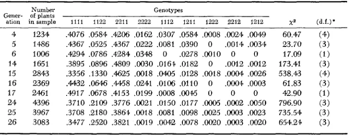
TABLE 3

Two-locus relative genotypic frequencies for locus pair A-B

Gener- ation 4 5 6 14 15 16 17 24 25 26 Number

of plants

in sample

1234 1486 1006 1651 2843 2369 2461 43 96 3967 3083 Genotypes

1111 1122 2211 2222 1112 1211 1222 2212 1212

.4CJ76 ,0584 ,4206 ,0162 ,0307 .0584 ,0008 ,0024 ,0049 ,4367 .0525 ,4367 ,0222 .Om1 ,0390 0 .0014 .0034 .4294 ,0786 ,4284 ,0348 0 ,0278 ,0010 0 0 ,3895 ,0896 .4809 ,0030 .016+ ,0182 0 .0012 ,0012 .3356 ,1330 ,4625 .0018 . M 5 ,0128 ,0018 . O W ,0026 .4432 .OM6 ,4468 ,0241 .0106 .0110 0 .OOO+ ,0003 ,4917 ,0678 .4153 .0199 .0008 ,0046 0 0 0 .3710 ,2109 ,3776 .a021 ,0150 .0177 .WO5 .OW2 ,0050 .3708 ,2180 .3864 .0018 .Om1 ,0098 .0025 ,0003 .0023 ,3477 .e520 .3821 .0019 ,0042 ,0078 .0020 .OW3 ,0020

60.47 23.70 17.09 173.41 538.43 61.83 42.90 796.90 735.54 654.24

TABLE 4

Two-locus relatiue genotypic frequencies for locus pair A-C

Number Genotypes

Gener- of plants

--

ation insample 1111 1122 2211 2222 1112 1211 1222 2212 1212 ~a (d.f.)*

4 1234

5 1486

6 1006

14 1651

15 2843

16 2369

17 2461

2E 4396

25 3967

26 3083

.3168 .I297 .3039 .I 159 .0494 .0356 .0065 ,0203 .0219 .2874 .I837 .3183 .I339 ,0262 .0162 .004f .0081 ,021 5 .3101 .I 958 .3042 .I541 ,0020 .0159 .0020 .0050 .0109 .3410 .1133 .3701 ,0878 .0412 .0170 .0012 .0272 .0012 ,2726 2279 .3394 ,1224 .Om5 .0137 .Om5 .0028 .0102 .2672 ,2356 ,3377 .I245 .0156 .0030 .WO4 .0080 .0080 ,2926 ,2662 ,3170 ,1154 .0016 .OW8 0 .0028 ,0016 .2543 .2807 ,2771 .0958 ,0619 .0139 ,0048 .0070 .OM

.2059 .3857 .2637 ,1230 ,0053 .0058 .0050 .0018 .0038 .I768 ,4220 .2809 .I015 .0052 .0036 .@I36 ,0019 .OM

76.80 278.04 21.21 15.40 128.68 119.23 113.77 430.45 422.08 569.61

* All x 2 values significant at P = .001

I n general we write the relative frequency of a quantity z as f(z)

.

For the two- locus genotypes then we have such frequencies as f(A1A1B2B2) and f(AIAIB,B,). On some occasions we need to take notice of which genes were received from the same gamete. For example for genotypes formed by the union of gametes AiBj and AI,Bz

(i,

j ,

k

and 1 are not necessarily different) we write the frequency as f(AiBj,AkBz) or even just as f(ij,kZ) when it is clear to which locus pair we are referring. Note that f(ij,kZ) = f ( k l , i j ) , so that heterozygote frequencies may be written as twice either of two equal quantities. For example we can write 2f(AlBl,AlB,) for f(A1B1,A1B2)

f

f (A,B,,A,B,) where both expressions equal

f

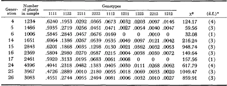
( AlAlBlB2). The coupling and repulsion double heterozygotes can not be dis- tinguished without progeny testing, and since this was impracticable, only the sum of these two classes is available. The generation time for all frequencies may be designated with a superscript.

TABLE 5

Two-locus relative genotypic frequencies for locus p ' r B-C

Gener- ation 4 5 6 14 15 16 17 24 25 26 Number of plants in sample 1234 1486 1006 1651 2843 2369 2461 4396 3967 3083 Genotypes

1 1 1 1 1122 2211 2222 1112 1211 1222 2212 1212 -

.6240 .I953 .0292 .0365 .0673 .0032 .0203 .OW7 .01%

.5935 .2719 ,0256 .0+51 .0471 . a 7 .0054 .OO# .0047 .5845 . 2 8 8 .0457 ,0676 .0169 0 0 .0010 0 ,6964 ,1386 ,0267 . a 3 9 ,0535 . W 9 .0097 .0121 . W 2 .6201 .I868 .0035 .I298 .0130 .OG21 .0362 .0032 .a053 .5801. .2980 ,0270 .0587 .0215 .W .0038 ,0030 .0072 ,5920 .3133 ,0195 .0683 .0061 .OOO8 0 0 0 .4941 2318 . M Z ,1383 .0405 ,0030 .0111 .Om8 .0062 ,4726 2.889 .0010 ,2180 ,0055 ,0018 .0069 .GO33 .0020 .4551 .2744 ,00155 ,2494 ,0081 .WO6 ,0032 .0010 .0027

Xa 124.17 59.56 32.08 216.24 948.74 149.64 157.56 617.79 1049.47 859.91 (d.f.1'

510 B. S . WEIR, R . W. ALLARD A N D A . L. KAHLER

TABLE 6

Two-locus relative genotypic frequencies for locus pair A-D

Number Genotypes

Gener- of plants

ation i n s a m d e 1111 llC2 2211 2222 1112 1211 1222 2212 1212 xa (d.f.)

5 1486 .2194 .2759 .1992 ,2591 .0020 ,0195 ,0229 .0020 0 0.21 (3) 6 1006 .2704 2316 2.336 .2286 .0060 .0159 ,0119 .0010 .0010 3.24 (3) 16 2369 .2684 ,2486 .2288 .241)2 .0013 .0059 .CO51 ,0013 .0004 2.66 (3) 17 2461 .3072 .2511 .2251 ,2044 ,0020 .0033 .0012 ,0057 0 10.29 (3)* 25 3946 .3876 .2051 2213 .1591 ,0050 .0091 ,0040 ,0043 .0015 23.26 (3)*** 26 3083 .@19 .1369 .2523 .1242 ,0052 ,0068 ,0039 ,0078 .0010 47.87 (3)***

* x 2 value significant P = .05, * * * P = ,001.

TABLE 7

Two-locus relative genotypic frequencies for locus pair B-D

Gener- ation

5 6 16 17 25 26

Number of plants in sample

1486 1006 2369 2461 3946 3083

Genotypes

1111 1122 2211 2222 I l l 2 1211 1222 2212 1212

.4004 .5081 .0310 .0437 .0040 .0067 .0061 0 0 .4642 .4145 ,0557 ,0576 ,0070 0 0 .0010 0 .4356 .@22 ,0621 ,0258 .0021 .0055 .0059 .OOO8 0

.4762 ,4283 .0593 .0281 ,0069 0 .ooo4. .W .WO4 ,4149 ,3431 .1979 .0226 .0089 ,0081 .0025 .OW0 0 ,4840 .21.13 2316 ,0227 .0123 ,0055 .0010 ,0016 0

xa (d.f.)

0.87 (2) 0.55 (1)

37.w (2)*** 18.55 ( l ) * * * 358.36 (3) ***

182.16 (3)***

* * * x 2 values significant at P = .001.

TABLE 8

Two-locus relative genotypic frequencies for locus pair C-D

Number Genotypes

Gener- of plants

ation insample 1111 1122 2211 2222 1112 1211 1222 2212 1212 xa (d.f.)

5 1486 ,2483 ,3708 ,1615 .1602 ,0027 ,0282 ,0269 .OW7 .WO7 14.92 (3)** 6 1006 ,3181 .3081 ,1889 .1590 .W .0129 .0050 ,0040 0 4.60 (3) 16 2369 .3182 .2879 .1718 .1887 .0017 .0131 .0173 0 ,0013 6.76 (3) 17 2461 ,3454 .2609 ,1861 .1938 .0061 .0041 .0020 .0016 0 18.26 (3)*** 25 3946 ,2525 ,2174 .3616 .1480 ,0048 ,0068 .0028 .0048 ,0013 123.36 (3)*** 26 3083 ,2997 .1524 ,4139 ,1087 .0091 .0075 ,0039 ,0045 .OW3 71.45 (3)***

~~ ~

* * x2 value significant at P = .01; * * * P = .W1.

Two-locus genotype frequencies are given in Tables 3 through 8. The tables for

the sixth o r seventh generation. Since no consistent changes occurred in the fre- quency of heterozygotes in the intermediate or late generations, this expectation also appears to have been realized in CCV.

For Loci A and B the A,B,/A,B, homozygote (12 allelic combination) in- creased at the expense of all other double homozygotes. Similar changes took place for the A and C, and B and C locus pairs with the A,C,/A,C, and B2C,/BzCz homozygotes increasing in frequency. Thus the initially most frequent allelic combinations were not those most favored by environmental conditions at Davis, California.

Similar general comments can be made for the unlinked locus pairs A-D, B-D and C-D. The main difference is that the level of heterozygosity is lower for these locus pairs in the early generations and that the level changes little over genera- tions. However, as discussed earlier (11)

,

this is almost certainly due to under- estimation of heterozygosity arising from inability to identify heterozygotes in- volving the DN allele. This allele does not produce a band in starch gels and, since it is recessive to alleles which produce bands, its heterozygotes are wrongly classi- fied as homozygotes.

A test for interactions between pairs of loci parallel to that used above for homozygous combinations can be made by comparing observed two-locus geno- typic frequencies with expectations calculated from one-locus frequencies. One- locus frequencies can be obtained from the data in Tables 3-8 by appropriate summations of two-locus frequencies. For example, the frequency of A,A, can be obtained from the A-B frequencies as: f(A,A,) = fAIAIBIB1)

+

f(A1A1B1B2) -k f (A,A,B,B,)

.

In more general notation, for the A locus:

Treating the products of one-locus frequencies [such as f ( AiAk) and f (BjBz) ] as the expected values of the observed two-locus frequencies [such as f ( AiAkBjBL)], we form the chi-square goodness-of-fit statistics shown in the right hand columns of Tables 3-8. Chi-square values have four degrees of freedom (there are eight independent two-locus frequencies, from which four independent one-locus fre- quencies have been estimated) except where it was necessary to combine classes to give expected values larger than three. Exact expressions for the expected dis- crepancies between two-locus frequencies and the product of corresponding one- locus frequencies for neutral alleles are given by

WEIR

and COCKERHAM (in preparation). These discrepancies, while remaining non-zero, tend to be very small quantities which would certainly give non-significant chi-square values; also the

x2

values are not expected to increase over generations with neutral al- leles. The

x2

values for the six pairwise comparisons between loci A, B, C, and D

all increase and are consistently significant by the middle or late generations, thus providing evidence that these loci are under selection.

512 B. S. WEIR, R . W. ALLARD A N D A. L. K A H L E R

organization of the two-locus zygotic arrays that has occurred over generations. Full data for observed and relative deviations are given for locus pair B-C in Table 9, where f o r convenience the deviations f(BiBkCjCL) - f(BiBk)f(CjCL) have been rounded to the nearest integer. It can be seen that there is a consistent excess of B,BICICl and B,B,C,C, and a consistent deficit of B,B,C,C, and B,B,C,C, double homozygotes (compare with Table 2, which gives data for 3 alleles/locus)

.

The deviations for the heterozygous classes are erratic due to sampling errors so that patterns are more difficult to identify. However, two of the singly heterozy- gous classes (B,B,C,C,,B,B,C,C,) and the double heterozygote ( BIB,C,C,) are in excess in most generations, while the other two singly heterozygous classes

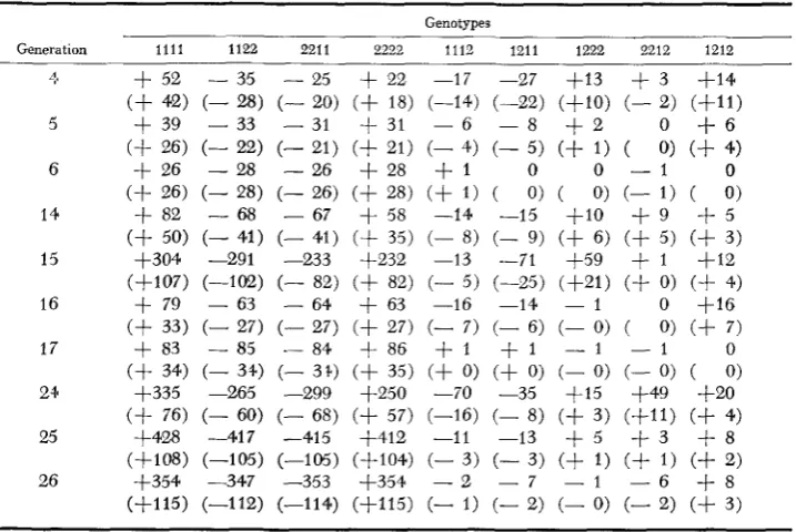
( B,B,C,C,,B,B,CICl) are in deficiency in most generations. This is a drastically different pattern from that expected for neutral alleles (WEIR and COCKERHAM, in preparation). Only part of the results (observed and relative deviations from expected numbers in generations 6, 17 and 26) are given for the other pairs of loci (Table IO) because these partial results are adequate to establish that similar complicated epistatic interactions also occur in each of these cases.

Another way of characterizing two-locus behavior in CCV is in terms of changes in the frequencies of gametic ditypes over generations. Gametic ditype

TABLE 9

Obserued deviations of two-locus numbers from products of one-locus numbers for locus pair B-C in three early, four intermediate, and three late generations of CCV. Relaiiue deuiations

[(obserued deuiution/N) x IOOO] are in parentheses*

Genotypes

x

Y

8

B

9)

514 B. S. W E I R , R. W. A L L A R D A N D A . L. K A H L E R

frequencies can be obtained from appropriate sums of genotypic frequencies. For example, for loci A and

B:

f(AiBi) = f(AiBi,AiBi) f f(AiBi,Aib)

+

f(AiBi,A,Bi) f f(AiBi&Bz) /(Ai&) = f(AiBz,AiBi) f f(AiBz.AiBz)

+

f ( A i B A B i )

+

f(AiB*,AJL) f(AJ%) = f(A$i,AiBi) -I- f(A2Bi,AiB2)

+

f(A,Bi,AzBi) f f(A&L,AzB,) f(A&) = f(AzBz.AiBi) f f(A,B,,AiB,) f f(A,B,,AJ%)

+

f(A&A&), and, in general,

f ( i j )

= f(ij,kZ). Estimation of the gametic frequencies re-

quires that all 10 genotypic frequencies be known but, as mentioned above, the experimental methods of the present study do not separate coupling from repul- sion double heterozygotes. However, we see from Tables 3-8 that the total fre- quency of double heterozygotes is always very low and often zero. Since each

f

(ij,kZ) and f (i2,kj)

,

where

i

#

k,

j #

Z,

is bounded by zero and the small quantity

1/2f(ikjZ) we expect good approximation to actual values in our sample if we set

f(ij,W

= f(il,kj) = ( 1 / 2 ) f ( i k , i O , [e.g. f(AlBl,A2B,) = f(A1B2,A2B1) = 1/4f

(AlAzBlB2)]. Hence this procedure was followed in computing the frequencies of gametic ditypes. The frequencies of gametic ditypes are not reported since they are very close to frequencies of double homozygotes, given in Tables 3-8.

However. we note that highly significant changes in the frequencies of the ga- metic ditypes occurred in a number of single-generation transitions. In many cases (e.g. AiBl in transition from generation 15 to 16 and AICz in transition from generation 24 to 25) changes in frequency of 10 standard errors or larger oc- curred. It is also clear that longer-term changes took place. As examples, the AIBz, AIC, and

BzC2

ditypes all more than tripled in frequency whereas A,C, and B,C,

decreased markedly in frequency over the 22 generation interval studied. Since many of the single generation and also long-term changes in gametic ditypes (and double homozygotes) are larger than can be accounted for by mutation, migration or genetic drift (11) they are evidently due to selection.

Gametic phase disequilibrium: The gametic phase disequilibrium parameter (also called linkage disequilibrium. epistatic disequilibrium, gametic phase un- balance, disequilibrium linkage function and linkage deviation function), A, defined as the deviation of observed gametic ditype frequencies from expected frequencies computed as products of allelic frequencies, provides still another measure of the changes which occurred in CCV. For example, gametic phase dis- equilibrium f o r loci A and B is given by

kl

A = f(AiBi) - f(Ai)f(Bi) = f(Ai)f(Bz) - f(AiBz)

= f(Az)f(Bi)

-

f(AzBi) 1 f(AzB2) -f(Az)f(Bz)

TABLE 11

Measures of gametic phase disequilibrium A (top figure), A’ (middle figure)

and r (bottom figure) for six two-locus pairs

Locus pair

Generation A-B A-C B-C A-D B-D C-D

Initial* 4 5 6 14 15 16 17 2% 25 26 -0.012 -0.250 -0.079 -0.572 -0.1 74

-0.015 -0.461 -0.112 -0.019 -0.354 -0.124 -0.047 -0.923 -0.308 -0.072 -0.954 -0.395 -0.021 -0.459 -0.141 -0.019 -0.483 -0.132 -0.959 -0.413 -0.086 -0.959 -0.421 -0.098 -0.965 -0.467 -0.025 -0.08 0.01 1 0.055 0.045 -0.006 -0.041 -0.025 -0.023 -0.136 -0.096 -0.012 -0.070 -0.050 -0.015 -0.128 -0.070 -0.046 -0.266 -0.192 -0.048 -0.270 -0.200 -0.051 -0.303 -0.21 1

-0.061 -0.372 -0.253 -0.078 -0.381 -0.320 -0.103 -0.493 -0.422 0.021 0.355 0.144 0.028 0.407 0.202 0.023 0.429 0.173 0.027 0.376 0.176 0.042 0.536 0.324 0.093 0.927 0.531

0 . a 8

0.483 0.201 0.034 0.633 0.219 0.065 0.503 0.318 0.105 0.963 0.503 0.114 0.942 0.522

0.002 0.001 0.009 0.037 0.008 0.010 0.008 0.004 0.032 0.063 0.032 0.024

0.008 -0.018 0.032 -0.377 0.031 -0.120 0.006 -0.012 0.027 -0.298 0.026 -0.086

0.016 -0.060 0.071 -0.709

0.024 -0.047 0.068 -0.297

0.146 -0.660 0.111 -0.238

--0.022 -0.112 -0.093 -0.008 -0.W - 0 . 0 3 5

0.01 1 0.060 0.047 0.019 0.084 0.076 -0.042 -0.21 7 -0.1 74 -0.032 -0.221 -0.14.4

~ ~ ~ ~

* A, A’ and r computed from gametic ditype frequencies in the parents of CCV, assuming no

change took place during the intercrossing phase of the synthesis of this population. It is unlikely that selection had much effect on A during this phase, since propagation was under space planting and survival was high. However, recombination almost certainly led t o a reduction in A during this phase, so that the values reported in this table are almost certainly overestimates of the actual gametic phase disequilibrium that existed in the initial generation.

estimated values of A.) Values of A are a function of gene frequencies and hence they have the disadvantage that they cannot be compared directly unless gene frequencies are equal. Values of A can, however, be adjusted for gene frequency

516 B. S. W E I R , R . W. ALLARD A N D A. L. K A H L E R

take near maximal values when allelic frequencies differ widely at pairs of loci. The correlation coefficient, T-, between alleles is less sensitive to differences in

allelic frequencies and has the additional advantage that its sampling distribution is known (Nr’

x2).

Consequently we have also reported T- values in Table 1 1. It

can be seen from this table that A, A’ and T-, although nonzero in the initial genera-

tion, were all small and perhaps not larger than expected due to the effects of sampling a small number of parents. Thereafter A increased rapidly, until in the latest generations, it had reached more than 90% of its theoretical maximum value for the tightly linked A-B and B-C locus pairs and nearly 50% of its maxi- mum value for tightly linked locus pair A-C. Substantial gametic phase disequi- librium had also developed for the three unlinked locus pairs by the late genera- tions, especially for locus pair B-D for which A exceeded 65

%

of its maximum in generations 25 and 26. The correlation coefficients, r, also indicate the develop- ment of substantial gametic phase disequilibrium, especially for the linked pairs of loci and for the B-D combination.

For a pair of adaptively neutral loci linked with amount h of linkage, it can be shown

(WEIR

and

COCKERHAM,

in preparation) that for a population practicing an amount s of selfing, the geometric rate of convergence of A to zero soon becomes

Thus, for the neutral situation, any original gametic phase disequilibrium that exists will be lost over generations, although in CCV with t = .0057 the rate of loss is expected to be low (< .4 percent/generation), even for pairs of unlinked loci. I n any event the absolute value of A is not expected to increase with neutral alleles. as the values in Table 11 are seen to do. Increasing absolute values of A

have been reported previously in experiments with both outbreeding (e.g. CANNON 1963) and inbreeding species (e.g. HARDING and ALLARD 1968). For random mating populations it can be shown that A may increase with tight link- age and selection (discussion in EWENS 1969). Although theory showing condi- tions under which gametic phase disequilibrium may persist (though not in- crease) has been restricted in inbreeding populations to adaptively neutral loci

(COCKERHAM and WEIR, in preparation), numerical results showing permanent gametic phase disequilibrium in the presence of selection have been reported by JAIN and ALLARD (1966). Analyses of changes in the gametic arrays thus support results of analyses of the zygotic arrays discussed above in indicating striking departures from the neutral situation in CCV. Since the effects of mutation, mi- gration and genetic drift are too small t o be measurable in this population (11) the observed changes are evidently due to selection. In the next section we esti- mate the selective values of the various genotypes to obtain a quantitative meas- ure of the intensity of this selection.

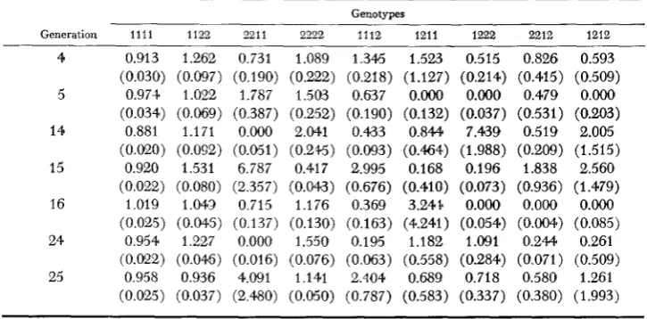
TABLE 12

Estimates of two-locus selective values and standard errors (in parentheses) for locus pair B-C

Genotypes Generation

4

5

14

15

16

24

25

I l l 1 1122 2211 2222 1112 1211 1222 2212 1212

0.913 1.262 0.731 1.089 1.345 1.523 0.515 0.826 0.593 (0.030) (0.097) (0,190) (0.222) (0.218) (1.127) (0.214) (0.415) (0.50)

0.974 1.022 1.787 1.503 0.637 O.OO0 0.000 0.479 O.Oo0

(0.034) (0.069) (0.387) (0.252) (0.190) (0.132) (0.037) (0.531) (0.203) 0.881 1.171 0.000 2.041 0.433 0.844 7.439 0.519 2.005

(0.020) (0.092) (0.051) (0.21.5) (0.093) (O.ffi4) (1.988) (0.209) (1.515) 0.920 1.531 6.787 0.417 2.995 0.168 0.196 1.838 2.560 (0.02.2) (0.080) (2.357) (0.043) (0.676) (0.410) (0.073) (0.936) (1.479)

1.019 1.044 0.715 1.176 0.369 3.24% 0.000 0.000 O.OO0

(0.025) (0.045) (0.137) (0.130) (0.163) (4.241) (0.054) (0.004.) (0.085) 0.954 1.227 0.000 1.550 0.195 1.182 1.091 0.244 0.261 (0.022) (0.04.6) (0.016) (0.076) (0.063) (0.558) (0.284) (0.071) (0.50)

0.958 0.936 4.091 1.141 2.404 0.689 0.718 0.580 1.261 (0.025) (0.037) (2.480) (0.050) (0.787) (0.583) (0.337) (0.380) (1.993)

illustrate some features of the estimates that were common to all locus pairs. First, the estimates for the heterozygous genotypes have large standard errors and are quite erratic due to sampling errors. The same is the case for the infrequent double homozygotes, e.g. B,B,C,C,. Second, values in successive generations are negatively correlated because they share a common set of genotypic frequencies, used once as f”+l(z) and once as f ” ( z ) (see 11). However, the estimates of selec-

tive values of the double homozygotes generally have small standard errors and these estimates reflect the observed trends in gametic and genotypic frequencies. For example, for loci B and C, the increase in B,B,C,C, at the expense of BIBIC,Cl is reflected by the generally larger selective values of the former. The picture for heterozygotes is obscured by sampling variation.

The selective values for loci B and C are typical in that they do not appear to change in response to change; in genotypic frequencies. For example, the selec- tive values for B,B,C,C, were much the same in early generations when the B,C, double homozygote was infrequent in the population as in later generations when its frequency had increased several fold. Thus general frequency-dependent selection featuring advantage of infrequent genotypes, i.e., w (z) increasing with decrease in f (z)

.

and vice versa, appears to be unimportant in CCV. On the other hand, nonlinearities that might arise from frequency-dependent selection appear in a number of cases. As an example. the selective values of B,B,C,C, are higher than those of BIB,C,C, even though the B,C, gamete is very infrequent in the population. This suggests a compensatory type of frequency-dependent selection. Of course all selective values were estimated from observed genotypic frequencies and so in this sense they are frequency dependent.

518 B. S . W E I R , R. W. ALLARD A N D A. L. K A H L E R

TABLE 13

Estimates of two-locus mean selective ualues and standard errors (in parentheses)

Locus pair 1111 1122 2211 2222 1112 1211 1222 2212 1212

A-B 1.011 1.062 0.969 2.507 1.151 0.985 3.285 1.151 1.031

A-C 0.902'' 1.266" 0.962 1.069 0.564. 1.057 1.223 1.448 2.997

B-C 0.946** 1.171" 2.016 1.274'' 1.197 1.036 1.423 0.641 0.954

A-D 1.070 0.818' 1.171' 0.824' 4.441 1.287 1.132 3.36-1. O.Oo0 (0.015) (0.067) (0.013) (0.919) (0.163) (0.122) (2.157) (0.163) (0.744)

(0.018) (0.036) (0.017) (0.036) (0.165) (0.181) (0.518) (0.383) (1.777)

(0.010) (0.027) (0.493) ( 0 . M ) (0.156) (0.644) (0.293) (0.176) (0.429)

(0.038) (0.031) (0.036) (0.029) (2.030) (0.266) (0.269) (1.531) (6.899) B-D 1.133' 0.809" 1.305 1.115 3.141 0.380; 0.379 1.458

-t

(0.024) (0.018) (0.124) (0.113) (1.043) (0.133) (0.193) (0.815)

-

C-D 1.164' 0.799' 1.110 0.901 4.378 1.136 1.195 7.296 0.000

(0.035) (0.025) (0.043) (0.040) (1.497) (0.195) (0.410) (7.035) (2.902)

' Significant departure from 1.000 a t P

<

0.05.

*' Significant departure from 1.000 a t P

<

0.01.

t

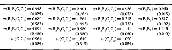
Non-estimable.

small standard errors and reflect the observed trends in genotypic frequencies. Although the selective values of specific heterozygotes are still erratic even when averaged over generations, heterozygotes tend to have higher selective values than double homozygotes. This is reflected in mean selective values of the double homozygotes and the heterozygotes (including double heterozygotes) which are

1.141 and 1.729 respectively. Thus averaged over all of the data of this experi- ment, the selective values indicate heterozygotes are about 52% superior to homo- zygotes in reproductive capacity.

In the course of deriving two-locus selection estimates, we also pick up one- locus selective values by taking appropriate marginal totals. For example, we obtain the post-selection one-locus frequencies for AiAk as

while (Appendix A) pre-selection frequencies are

so that the selective values for Ai& are given by w"(AiAk)=g"(AiAk)/f" (AiAk). The values f o r locus B may be obtained similarly. A sample of these marginal values, for loci B and C, are given in Table 14. The single-locus and two-locus estimates bear little relationship to each other in this case, and also for the other locus pairs, as expected considering the complex epistatic nature of the selective forces.

D I S C U S S I O N

T A B L E 14

Estimates of one- and two-locus selective values and standard errors (in parentheses)

for locus pair B-C in generation 25

w (BIB,C,C,)= 0.958 (0.025) w(B,B,C,C,)= 0.689

(0.583) w(B2B,C,C,)= 4.091

(2.480) w(C,C,)= 0.964

(0.025)

w(B,B,C,C,)= 2.404

w(B,B,C,C,)= 1.261

w(B,B,C,C,) = 0.580 (0.787)

(1.993)

(0.380)

(0.313) w(C,C,)= 1.64.0

w(B,B,C,C,)= 0.936 w ( B I B 1 ) = 0.960

w(B,B2C,C2)= 0.718 w(B,B,)= 0.817

w(B,B2C,C,)= 1.141 w(B,B,)= 1.146

(0.037) (0.013)

(0.337) (0.192)

(0.050) (0.049)

w(C,C,)= 1.020 (0.024)

operation of selection. Pairs of adaptively neutral loci which are in gametic phase equilibrium ( A = 0) are not expected to develop gametic disequilibrium (A # 0)

(WEIR and COCKERHAM, in press). With adaptive neutrality the frequency of gametic ditypes is also not expected to change i n a population such as CCV in which genetic drift, migration and mutation have only trivial effects (11). Yet i n CCV highly significant changes occurred in the frequencies of gametic ditypes, and striking gametic phase disequilibrium developed within a few generations for each of the six pairwise combinations of loci which were monitored. These results provide strong evidence that all four of the loci studied, or the linkage blocks they mark, have significant effects on survival.

The data also provide information concerning the complexity of the units on which selection acts in CCV. The A locus, due to the nature of its linkage relation- ships with Loci B and C, is particularly informative concerning the effects of selection on single loci. These three loci are ordered B ~ 0 . 0 0 2 3

*

A 0.0048

*

C.

Since no genes have been reported that occupy a shorter segment of chromosome than that estimated for Locus A (BENZER 1955), it seems likely that no locus other than A occurs between Loci B and C. Thus it is evidently the A locus itself, and not undetected genes linked to this locus, that produces the selective effects associated with the A system. Moreover, these effects are substantial indicating that single enzyme loci can have effects on survival of the same order of magni- tude as loci which govern some of the more conspicuous visible polymorphisms. The data also make it clear that selection operates not only on individual loci but that it also operates differentially on specific two-locus allelic combinations. The development of non-random associations in the gametic and zygotic arrays of both linked and unlinked pairs of loci is evidently attributable to interactions between selection and restriction of recombination resulting from linkage and/or inbreeding. Another feature of selection is that each allele at any one locus inter- acted favorably with at least one allele and unfavorably with at least one allele at each of the three other loci; thus complicated epistatic interactions occur not only at the two-locus level but, since each locus affects each other locus, also at the three and four locus levels, as shown more precisely by CLEGG, ALLARD and

520 B. S . WEIR, R. W . ALLARD AND A. L. KAHLER

LITERATURE CITED

ALLARD, R. W., A. L. KAHLER and B. S. WEIR, 1972

BENZER, SEYMOUR, 1955

CANNON, G. B., 1963

CLEGG, M .T., R. W. ALLARD and A. L. KAHLER, 1972

COCKERH~M,

c.

CLARK and B.

s.

WEIR, 1972 EWENS, W. J., 1969

HARDING, J. and R. W. ALLARD, 1968

The effect of selection on esterase allo- zymes in a barley population. Genetics 72: 4439-503.

Fine structure of a genetic region in bacteriophage. Proc. Natl. Acad. Sci. U.S. 41 : 3444-3544.

The effects of natural selection on linkage disequilibrium and relative fitness in experimental populations of Drosophila melanogaster. Genetics 48: 1201-1216.

Is the gene the unit of selection?: Evidence from two experimental plant populations. Proc. Natl. Acad. Sci. U.S., in press.

Descent measures for two loci with some appli- cations. (In preparation).

Population Genetics. Methuen and Company, London.

Population studies in predominantly self-pollinated species. XII. Interactions between loci affecting fitness in a population of Phseolus Zunatus. Genetics

61: 721-736.

The effects of linkage, epistasis, and inbreeding on popu-

The genetics of isozyme variants in barley. I. Esterases.

The interaction of selection and linkage. I. General considerations;

Mixed self and random mating at two loci (In S. K. and R. W. ALLARD, 1966

lation changes under selection. Genetics 53 : 633-659.

Crop Science 10: 44.1-4.18.

heterotic models. Genetics 49: 4Q-67. WEIR, B. S. and C . CLARK COCKERHAM, 1972 KAHLER, A. L. and R. W. ALLARD, 1970

LEWONTIN, R. C., 1965

preparation).

APPENDIX A

ESTIMATION O F TWO-LOCUS SELECTIVE VALUES

Estimation of two-locus selective values has received little attention, particularly when linkage and inbreeding are taken into account. (The methods given by TURNER 1967, 1968) are not general because his expressions for frequencies of double heterozygotes in inbreeding populations hold only for zero gametic phase disequilibrium (linkage disequilibrium), see COCKERHAM and

WEIR, in preparation). Here we extend the maximum likelihood estimators based on genotypic recurrence formulae (ALLARD and WORKMAN 1963) that were used to make the one-locus esti- mates (11). We develop the theory in some detail to show the necessity for certain assumptions. The method rests on comparing two sets of genotypic frequencies, one estimated prior to selection and the other estimated after selection has occurred. The selection model we adopt is Model I1 of WORKMAN and JAIN (1966). Our frequency data are obtained very early in each generation (from seven-day-old seedlings) and so measure genotypic frequencies shortly after the formation of zygotes from gametes of the mature individuals of the previous generation. We assume that the outcrossing which occurs between different individuals in the population is a t

random. This assumption appears to be reasonable in view of the finding (11) that outcrossing is homogeneous over genotypes in CCV. We also assume that no selection occurs between mating of the mature individuals in one generation and scoring of seedlings in the next generation and, thus, that all selection occurs between scoring and the mating of mature individuals in that generation. This assumption also appears to be reasonable because more than 99% of flowers produced kernels and more than 99% of kernels produced assayable seven-day-old seedlings. Comparing genotypic frequencies fn (z) of seedlings with genotypic frequencies g n (z) of mature individuals of genotype z in generation n therefore gives a measure of the relative selective values for this genotype. These selective coefficients are defined as

so that f"(2) and g n ( z ) may be called the pre- and post-selection frequencies respectively. Under

this model, seedling frequencies in generation n+l are determined solely by the mating system and frequencies of mature individuals in generation n. We thus have a functional relationship of the form

{f"+l(Z)} = * ( { g " ( z ) } ) .

{g" (2) } = +-I(

{P

+1(2) } ) 9

By equating these expected f"+l(z) values to their observed values (generation n+l seedling frequencies), the solution to

where +-I has the observed values substituted, gives the maximum likelihood estimates of the

g" (2). The problem then is to find +-I.

We proceed by first displaying the transition equations. Although we use the symbols A and B, these equations clearly apply to any pair of loci linked to an extent 1, and just as clearly to any number of alleles a t each locus. For loci A and B we suppose there are alleles Ai and Bj. As before, the frequency of genotypes formed by the union of gametes A,Bi and A,B, is written as f" (ij,kl)-meaning pre-selection frequencies in generation n. The corresponding post-selection frequency is written as g" (ij,kl). If we set

then the transition equations become:

for I # j .

These equations are for double homozygotes, homozygotes at the B locus only, homozygotes at the A locus only, and double heterozygotes, respectively. T h e divisor G =ZZZZ g"(i;,kZ) ensures that the pre-selection frequencies in generation n f l sum to one, and so are relative frequencies. If the generation n post-selection frequencies are also to be relative, then G = 1 and it will be taken as such. Note that G = zzzz w n ( i j , k l ) P(ij,kZ) also, so that G = fi, the

"mean fitness" of generation n. We have immsed unit mean fitness on our population. Another consequence is that

FT

u"(ij) = 1, so that by adding appropriate equations to obtain the pre- selection gametic frequencies in generation n+l :

ijkl

;jkl

11

f"+I(AiBj) =ZI:f"+l(AiB~,A,B,) = sun(ij)

+

tun (ij) = u "( i j ) ,

522 B. S. WEIR, R. W. ALLARD A N D A. L. KAHLER

so that the quantities u n ( i j ) are equal to these gametic frequencies and are thus observable. This leads us to define new functions of the observed generation n f l pre-selection frequencies:

hn+l(AiB,.,AkBz)

='

{ f @ + l ( A i B j , A k B l )

-

t P + l ( A i B , ) f " + l ( A , B Z ) } , s # 0

S

and to write the transition equations in the form:

hn+l(ii,ij) = p ( i j , i j )

+

I / 2 p z i g"(ij,pj)

+

1/2 2 gn(ii,iq)

QZI

k # i

l # i

k # i,. 1 # i.

This system of equations, which may be summarized as

{ h f l + W } = @{gYz)},

has the advantage over the system cp of being linear, and hence easy to transform to the system

{g"(z)} = O - l { h n + l ( z ) } .

The equations of this inverse system follow, where the hn+l(z) refer to their observed values,

SO that the g n ( z ) are maximum likelihood estimates (BAILEY 1951). Note that for free recombi-

nation (A=O) both double heterozygotes for any four alleles have the same coefficient in the

transition equations, so that we cannot find both of g"(ij,kl) and gn(iZ,kj) but only their sum.

{gn(ij,kZ)

+

gn(iZ,kj)

1

A

4 { h n + l ( i i , k ~ )

+

hn+l(il,kj)

1

k # i, 1

+

i.

selection frequencies can be determined, we can estimate all ten post-selection frequencies in the previous generation (although they are constrained to sum to one). In the present case there

are just nine observable genotypes, and while we could still estimate ten post-selection frequencies we note that the t w o double heterozygote frequencies are constrained to have a difference depending on the amount of gametic phase disequilibrium. We thus present just nine post- selection frequencies also-by taking the sum:

4

1+X*

{gn(ij,kZ)

+

gn(iZ,kZ)} =

-

{hn+l(ij,kZ)

#+

h"+l(iZ,kj)} for all A.

We stress, however, that setting both pre-selection double heterozygote frequencies equal to each other neither requires nor implies that corresponding post-selection frequencies, and hence selec- tive values, are equal unless gametic phase equilibrium prevails.

Once the p ( z ) are estimated, we need only divide by the corresponding f"(z) in order to estimate the selective value f o r the z t h genotype. Should the value of some fn(z) be zero, the

selective value is not estimable. Should a g"(z) be negative (as will happen if fewer of that genotype are observed in generation n+l than the amount of outcrossing alone would require), we say that the selective value of that genotype is zero. Both of these situations occurred occa- sionally for heterozygotes, presumably as a result of sampling error.

The selection coefficients wn(z) are functions of f n ( z ) , f n f l ( z ) , t and A. The estimates we have of all these quantities are subject to sampling error, and we can give estimates of the variance of each of the estimates (see Appendix of 11). We can, therefore, estimate the variance of w n ( z ) from these variances by using large sample theory (CRAM~R, 1946). To the order of accuracy of each of the estimates of f"(x), f"+l(z), t and A:

where

and all quantities are taken a t their estimated o r observed values.

An alternative method of treating the case of two alleles at each of two tightly-linked loci is to assume that the two pairs of alleles represent four alleles at a single locus. This treatment for locus pairs A-B, A-C and B-C gave selective values within 0.02 of those found as above. The mechanics of obtaining such estimates have been described previously (11).

LITERATURE CITED

ALLARD, R. W. and P. L. WORKMAN, 1963 Population studies in predominantly self-pollinated species. IV. Seasonal fluctuations in estimated values of genetic parameters in lima bean populations. Evolution 17: 470-480.

Testing the solubility of maximum likelihood equations in the routine application of scoring methods. Biometrics 7 : 268-274.

BAILEY, N. T. J., 1951

CRAM~R, H., 1946

TURNER, J. R. G., 1967 On supergenes: I. The evolution of supergenes. Am. Naturalist 107:

195-221.

-

, 1968 On supergenes: 11. The estimation of gametic excess in populations. Genetica 39: 82-93.

WORKMAN, P. L. and S. K. JAIN, 1966 Zygotic selection under mixed random mating and self Mathematical methods of statistics. Princeton.