Söldner-Rembold, Isabella (2018): The velocity ellipsoid of elliptical galaxies. Dissertation, LMU München: Fakultät für Physik

(1)

The Velocity Ellipsoid of Elliptical

Galaxies

Isabella S¨

oldner-Rembold

(2)

(3)

The Velocity Ellipsoid of Elliptical

Galaxies

Isabella S¨

oldner-Rembold

Dissertation

an der Fakult¨

at f¨

ur Physik

der Ludwig–Maximilians–Universit¨

at

M¨

unchen

vorgelegt von

Isabella S¨

oldner-Rembold

aus M¨

unchen

(4)

(5)

List of Figures

2.1 Velocity Ellipsoid Diagram. . . 22

2.2 Extended photometry of NGC 4660. . . 23

2.3 Original and four-fold symmetrised ATLAS3D _{kinematic data. . . .} ₂₈

2.4 ATLAS3D _{and 2D SLUGGS kinematic data. . . .} ₂₉

2.5 NGC 4660 internal Kinematics of initial models for NMAGIC. . . 34

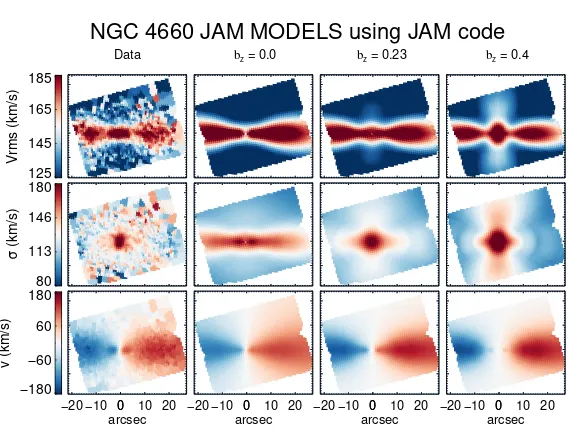
2.6 NGC 4660 internal kinematics of initial models for NMAGIC (c(R,z) and βz) 35 2.7 JAM method models of NGC 4660. . . 42

2.8 NGC 4660 projected kinematics of NMAGIC data-driven models . . . 43

2.9 NGC 4660 internal kinematics of NMAGIC data-driven models . . . 44

2.10 NGC 4660 projected kinematics of NMAGIC cross-driven models. . . 45

2.11 Comparison of NGC 4660 vrms data and models. . . 45

2.12 NGC 4660 internal kinematics of models with global βz as an observable. . 46

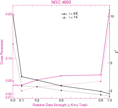
2.13 NGC 4660 internal kinematics of NMAGIC models with diﬀerent RDS. . . 46

2.14 NGC 4660 χ2 _{and cross parameter} _c 30 for models with diferent RDS. . . . 47

2.15 NGC 4697 JAM velocity ﬁeld models. . . 47

2.16 Comparison of NGC 4697 vrms data and models. . . 48

(10)

2.18 The normalized cross term cR,z and z-anisotropy of NGC 4697. . . 49

2.19 NGC 4697 χ2 _{and cross parameter} _c 30 for diﬀerent RDS. . . 51

2.20 Dark matter JAM models of NGC 4697 reduced χ2 _{. . . .} ₅₂

2.21 Dark matter JAM models of NGC 4697 ∆χ2 _{. . . .} ₅₃

2.22 The median anisotropy βz with dark matter halo . . . 53

2.23 The Mass-to-Light Ratio with dark matter halo. . . 54

2.24 The total density slopes of the diﬀerent stellar and dark halo models A-K. 58 2.25 The entropy S and the change of entropy with time δS/δwi. . . 60

2.26 Characteristics of negative particle models. . . 62

2.27 Histogram of the negative weights in models where the JAM condition is enforced. 63 2.28 Internal Kinematics of models with global target βz = 0.29. . . 64

2.A.1The MGE photometric data of NGC 4660 from Scott et al. (2013). . . 72

2.A.2 The major axis surface brightness proﬁle of NGC 4660. . . 72

2.A.3Contours of the Photometry of NGC 4660. . . 73

2.A.4The major axis surface brightness profile of NGC 4660 in the transition region. 75 2.A.5The original composite image of NGC 4660, MGE fit and residual between the two. 76 2.A.6The major axis surface brightness profile of NGC 4660. . . 78

2.A.7Normalisation of the S´ersic proﬁle of NGC 4660. . . 79

2.B.1Velocity of the NGC 4697 ATLAS3D _{data in kms}−1 _{vs radius.} _{. . . .} ₈₁

2.B.2Diagram of a kinematic ﬁeld where the major axis is aligned with the y-axis. 82 2.B.3Original ATLAS3D _{Data. . . .} ₈₃

2.B.4Shifted and Recentered ATLAS3D _{Data. . . .} ₈₃

2.B.5Four-fold symmetrised ATLAS3D _{data. . . .} ₈₄

(11)

LIST OF FIGURES xi

2.B.7The 2D SLUGGS kinematic data, velocity, σ, h3 and h4. . . 86

2.B.8Velocity Ratio of SLUGGS and ATLAS3D_{. . . .} ₈₈

2.B.9The 2D SLUGGS kinematic data, velocity, velocity dispersion, h3 and h4. . 89

2.B.10Transition between ATLAS3D _{and SLUGGS. . . .} ₉₀

2.B.11Transition between ATLAS3D _{and SLUGGS. . . .} ₉₁

2.B.12Gaussian Noise for velocity, σ, h3, and h4. . . 92

2.D.1NGC 4697 MGE Photometry . . . 96

2.D.2The 2D probability of the parameters M/Land z- anisotropy in JAM Jeans Models. 98 2.E.1Kinematics of diﬀerent data-driven halo models. . . 99

2.E.2Kinematics of diﬀerent cross-driven halo models. . . 100

2.E.3Comparison of ATLAS3D _{kinematic data of NGC 4660. . . 101}

2.E.4The circular velocity of NGC 4697 . . . 102

2.E.5Internal Kinematics of NGC 4697. . . 103

2.E.6Internal Kinematics of NGC 4697 (JAM assumption and photometry) . . . 104

2.E.7NGC 4697 Internal Kinematics Tension. . . 105

2.E.8NGC 4697 Internal Kinematics Tension (diﬀerently weighted γ) . . . 106

2.E.9Comparison to 1D SLUGGS data (Kinematics Only). . . 107

2.E.10Comparison to 1D SLUGGS data (Cross Only). . . 108

2.E.11Comparison to 1D SLUGGS data (Kinematics + Cross). . . 109

1 The x,z, and y-views of a triaxial particle model in NMAGIC. . . 113

2 Internal kinematics of a triaxial NMAGIC model. . . 114

3 Surface brightness in V-band of M87. . . 117

(12)

5 Surface density projection of M87. . . 120

6 Velocity dispersion of M87 NMAGIC models. . . 121

7 Anisotropy of M87 NMAGIC models. . . 122

1 Surface brightness proﬁle of NGC 4278. . . 127

2 Velocity distribution of NGC 4278 PNe. . . 128

3 Line-of-sight velocities of PNe of NGC 4278 and NGC 4283. . . 128

4 Azimuthally averaged vrms data of NGC 4278. . . 130

5 HI circular velocity data from Morganti et al. (2006). . . 138

6 Jeans model to vrms of NGC 4278 with diﬀerentrvir. . . 141

7 Jeans model to vrms of NGC 4278 with diﬀerent concentrations. . . 142

8 Jeans model to vrms of NGC 4278 with diﬀerentβ2. . . 143

9 Phase space diagram of GCs and PNe around NGC 4278. . . 144

10 Spatial distribution of PNe and GCs around NGC 4278. . . 145

(13)

List of Tables

2.1 Characteristics of initial models into NMAGIC for NGC 4660 and NGC 4697. 39

2.2 Properties of the dark matter halo models. . . 59

2.3 Characteristic parameters of the models of NGC 4660. . . 67

2.4 JAM ﬁt parameters to the ATLAS3D data of NGC 4660 and NGC 4697. . . 68

2.5 Characteristic parameters of the models of NGC 4697. . . 69

2.A.1S´ersic parameters of NGC 4660. . . 79

2.A.2MGE ﬁt parameters. . . 80

1 Properties of NGC 4278 and NGC 4283. . . 131

2 Dark matter fraction of NGC 4278 for diﬀerent models. . . 139

3 Jeans models parameters for NGC 4278. . . 139

(14)

(15)

Zusammenfassung

In der vorliegenden Arbeit wurde die Ausrichtung der Geschwindigkeitsellipsoide der ellip-tischen Galaxien NGC 4660 und NGC 4697 mit Hilfe des NMAGIC “Made-to-Measure” Modells untersucht. Als Daten wurden ATLAS3D _{and SLUGGS kinematische Daten}

ver-wendet. Die häufig verwendeten anisotropischen Jeans-Modelle (JAM) machen die An-nahme hvRvzi= 0. Es wurde daher untersucht, ob zylindrisch ausgerichtete Geschwindig-keitsellipsoide (_hvRvzi = 0) in elliptischen Galaxien mit realen Verteilungsfunktionen vorhanden sein können. Wir finden, dass es keine physikalischen Modelle von NGC 4660 und NGC 4697 mit gleichzeitiger globaler Anisotropie und zylindrisch ausgerichteten Ge-schwindigkeitsellipsoiden gibt. Modelle, für die die Orientierung des Geschwindigkeits-ellipsoids keine Rolle spielen, sind die einzigen Modelle mit realen Verteilungsfunktionen und zylindrisch ausgerichteten Geschwindigkeitsellipsoiden. Die Qualität von Modellen mit _hvRvzi = 0 hängt daher davon ab, wie isotrop die interne Struktur der zu mode-lierenden Galaxie ist. Wir untersuchen den Einfluss dieser Einschränkung auf das Masse-Licht-Verhältnis und den damit verbundenen Anteil dunkler Materie. Eine Untersuchung verschiedener Verteilungenen von dunkler Materie in NGC 4697 zeigt, daß ein Halo von dunkler Materie im intermediären Massenbereich die kinematischen Daten bis zu einem effektiven Radius von 1.5Regut reproduziert, wenn die Ausrichtung der Geschwindigkeit-sellipsoide nicht eingeschränkt wird. Mit der Bedingung zylindrischer Ausrichtung dagegen läßt sich kein gutes Modell für die Kinematik konstruieren. Die Qualität der Modelle nimmt dabei mit ansteigender Dunkler-Materie-Halo ab.

(16)

ergibt sich, dass die Gesamtmasse gut durch eine Dichteverteilung der Form ρ ≈ rγ _mit einem Faktor γ =₋2.1 beschrieben wird.

Um die kinematische Struktur der Galaxie NGC 4283 in der Nachbarschaft von NGC 4278 zu untersuchen, benutzen wir ebenfalls PNe. Die PNe der Galaxien sind klar ge-trennt aufgrund der verschiedenen mittleren Geschwindigkeiten von (622_±21) kms−1 _f¨_ur

NGC 4278 and (1050±21) kms−₁

(17)

Abstract xvii

Abstract

We present an investigation into the alignment of velocity ellipsoids in the elliptical galax-ies NGC 4660 and NGC 4697 using the NMAGIC Made-to-Measure Dynamical Modelling approach, with ATLAS3D _{and SLUGGS kinematic data. We test whether cylindrically}

aligned velocity ellipsoids (hvRvzi = 0), assumed by the widely used Jeans Anisotropic Models (JAM), can be present in elliptical galaxies with real distribution functions. We find that there are no physical models of NGC 4660 and NGC 4697 with both global anisotropy and cylindrically aligned velocity ellipsoids. The only models with real distri-bution functions and _hvRvzi= 0 are found to be isotropic models, where velocity ellipsoid orientation is irrelevant. The quality of models with _hvRvzi= 0 is therefore dependent on the similarity of their internal structure to isotropy. We probe the effect of this limitation on Mass-to-Light Ratio and dark matter content. A study of several dark matter distri-butions of NGC 4697 finds that an intermediate dark matter halo reproduces kinematic data well to 1.5 Re when the alignment of velocity ellipses is left unconstrained. Whilst constrained to have cylindrical alignment, no good quality models to the kinematics are found, with quality of models decreasing with increasing dark matter halo.

We investigate the dark matter distribution and orbit distribution of the intermediate elliptical galaxy NGC 4278 using spherical Jeans modelling and HI rotation data. We use planetary nebulae as tracers beyond the point that stellar light becomes too faint for absorption line spectroscopy. Combing the vrms of the PNe with that of SAURON IFU data, we compute a profile to which the Jeans models are made. The HI rotation curve provides a constraint on the total potential of the galaxy. NGC 4278 is an interesting target as it has a flat root-mean-square velocity which is more characteristic of a large mass elliptical galaxy. Using our models to decompose the potential into stellar and dark matter, we find that NGC 4278 is consistent with the models with a considerable amount of dark matter. Additionally the total mass is well reproduced by a total power law density ρ_≈rγ_{, with} _γ ₌₋₂_._{1, which points to an accretion history.}

The PNe additionally trace a galaxy nearby to NGC 4278 named NGC 4283. The planetary nebulae of the galaxies are well separated using the mean velocities at (622_±21) kms−₁

for NGC 4278 and (1050 ±21) kms−₁

(18)

(19)

Chapter 1 Introduction

1.1 Dark Matter

The visible matter in the Universe is made of gas, stars, and dust. The amount of visible matter is not suﬃcient, however, to explain the gravitational forces present in the Universe. One type of models that can explain the presence of excess matter postulates the existence of dark matter, which interacts only gravitationally but is invisible to the electromagnetic force.

There are several diﬀerent types of astronomical evidence for the existence of dark mat-ter. Historically, the earliest evidence was the observation by Oort (1932) that the velocities of nearby stars are too high given their mass. Zwicky (1933) measured the velocity dis-persion of a galaxy cluster and concluded that the disdis-persions imply a factor of 10 to 100 more mass than the visible matter contained in the galaxy. Zwicky (1933) concluded that this could be explained by some form of invisible matter (Trimble, 1987).

Subsequent work by Babcock (1939) on the M31 galaxy, Ostriker et al. (1974) and Rubin et al. (1978) on spiral galaxies, and Einasto et al. (1974) on galaxy clusters showed through the analysis of rotation curves that galaxy mass increases in the region beyond radii that the visible matter would indicate. Further astronomical evidence for dark matter has been found using gravitational lensing (e.g Wu et al., 1998; Natarajan et al., 2017) and the measurement of the Cosmic Microwave Background (CMB, Ade et al., 2016).

While there is indirect evidence for the existence of dark matter, experiments have so far failed to directly detect dark matter interactions, theorised, among others, to be weakly interacting massive particles (WIMPs, Liu et al., 2017).

(20)

beginning of the Universe. The Universe evolved from an extremely hot and dense state according to the current standard model, suitable for the emergence of subatomic particles and their subsequent fusion into nuclei. As Hubble (1929) first discovered, the Universe is expanding, cooling as it expands. The discovery of Cosmic Microwave Background supports this view, first detected by Penzias & Wilson (1965). The CMB is a low temperature black body radiation, first measured using NASA’s Cosmic Background Explorer (COBE), with a temperature of ∼ 2.73 K (Smoot et al., 1992). It originates from the epoch of recombination, at the time in the evolution of the Universe where ionised electron-proton plasma recombined to form hydrogen.

Following the COBE map, there have been more measurements of the CMB performed by the Degree Angular Scale Interferometer (DASI Kovac et al., 2002), by BOOMERanG (Masi, 2002), and the WMAP (Bennett et al., 2013) and Planck Collaborations (Ade et al., 2016). The temperature ﬂuctuations in the CMB have been found to be very small and Gaussian on all scales (Komatsu, 2003; Ade et al., 2016).

Small anisotropies in density and temperature existed at the beginning, where the small perturbations in density later form the observed structures of the Universe, such as large scale structures, galaxies and clusters. This occurs during the inflationary epoch, where the Universe expands rapidly (Guth, 1981; Peacock, 1999). Numerical simulations such as the Millennium Simulation (Springel et al., 2005) give a picture of how dark matter structures formed from the density perturbations. The development of structures is hierarchical, with smaller structures merging into larger structures. These simulations are used to find relationships between the density and halo radius, such as the NFW profile (Navarro et al., 1996):

ρNFW(r) =

ρs

(r/rs)(1 +r/rs)2

, (1.1)

where rs is a scale length, and ρs is a characteristic density.

1.2 Elliptical Galaxies

(21)

1.2 Elliptical Galaxies 3

to for example the Milky Way disk.

We primarily deal with ETGs in this thesis, as we probe a dynamical modelling method (Cappellari, 2008) which has been applied to large samples of ETGs in, for example, ATLAS3D _{(Cappellari et al., 2011) and SAMI (Scott et al., 2015). It has also been}

ap-plied to samples with both ETGs and spirals in MaNGA (Li et al., 2018). Since the less complicated potential structure of ETGs is easier to model dynamically, we have chosen elliptical galaxies as our test cases. Due to the large number of stars typically present in an elliptical galaxy, approximately 109 _{to 10}11_{, spread over a large area of the order of tens}

of kiloparsecs (kpc), the density of such galaxies is low.

Surface Brightness

Elliptical galaxies generally have a bright central nucleus, with surface brightness decreas-ing rapidly with increasdecreas-ing radius. There are several methods to characterise the surface brightness proﬁles of elliptical galaxies. One example is the proﬁle from Sersic (1968):

I(R) =Ieexp −bn

" R Re

1/n

−1

#!

, (1.2)

where n is the Sérsic index, Ie is the intensity at the effective radius Re that encloses half the light of the galaxy, and bn is a factor dependent on n. A double-component Sérsic profile parametrisation from Hopkins et al. (2009), allowing more complex photometry, is given by:

Itot=I′exp −b′n

r

Rinner

1

n′_s!

+I0exp bn

r

Router

1

ns!

, (1.3)

where Rinner and Router are the effective radii of the inner and outer profile, n′s and ns are their Sérsic indices, and I′

and I0 are the normalisations. The parameters n′s and ns are ﬁxed to n′

s = 1.0 and ns = 1.88, given by Hopkins et al. (2009), while the eﬀective radii and normalisation are ﬁtted. The parameterbnis computed using the equation from Ciotti (1991):

Γ(2n) = 2γ(2n, bn), (1.4)

where Γ and γ are the complete and incomplete Gamma functions, respectively.

Kinematics

(22)

along the of-sight is observed. These lines are Doppler-shifted according to the line-of-sight velocities (Binney & Merrifield, 1997). The velocity profiles gathered from these measurements can be fit by a Gaussian function, which gives the mean velocity and ve-locity dispersion, and the Gauss-Hermite moments that describe the veve-locity profiles as a polynomial function defined as:

un(w) = (2n+1πn!)−

1

2H

n(w)e−w

2

/2_, _(1.5)

where w= (v₋ˆv)/σˆ and Hn(w) are the Hermite (Hermite, 1864) polynomials.

The Gauss-Hermite moments allow deviations from a pure Gaussian function. Since stel-lar velocity profiles often deviate from Gaussian functions, this feature can be an advantage. The fitted velocity ˆv and velocity dispersion ˆσ are different and can also differ from the mean v and σ (Bender et al., 1994). The commonly used third and fourth moments, h3

and h4, represent the skew and kurtosis of the velocity proﬁle, respectively.

Gauss-Hermite velocity profiles have been used effectively to break the mass-anisotropy degeneracy. The mass-anisotropy degeneracy appears because the information on the line-of-sight velocity and dispersion is consistent with multiple combinations of potentials and anisotropy profiles for a galaxy. For example, outside the centre of a galaxy a radial anisotropy decreases the velocity dispersion profile of the galaxy. Adding more mass to the gravitational potential, by either increasing the mass-to-light ratio or increasing the amount of dark matter, increases the velocity dispersion profile. The galaxy is therefore consistent with a higher potential and anisotropy, or with a lower potential and lower anisotropy. Both scenarios match the same data (e.g. Gerhard, 1993; Merritt, 1993; Saglia et al., 1997).

Gerhard (1993) concludes that the shape of the velocity profiles, quantifiable by the Gauss-Hermite moments, depends strongly on the anisotropy of the system and less on the stellar density and potential. The shape of the velocity profiles therefore constrains the anisotropy. Using this anisotropy and the velocity dispersion profile then constrains the other possible variables such as the potential.

Planetary Nebulae as Kinematic Tracers

(23)

1.3 Collisionless Galaxy Dynamics 5 Galactic matter and potentials

The gravitational potential of a galaxy combines all the different components of matter that are present, which are stellar and gas. In addition, it is theorised that dark matter represents a third component contributing to the potential. The amount of stellar matter present in the galaxy is derived from the luminosity of the galaxy, with a conversion factor known as the mass-to-light ratio (M/L), which determines how much of the light seen is due to matter. The mass-to-light ratio can be obtained using different methods, one using dynamical modelling of the velocity dispersion to find the best fitting potential. Another method is stellar population modelling (e.g. Binney & Merrifield, 1997).

1.3 Collisionless Galaxy Dynamics

Elliptical galaxies can be approximated as gravitationally bound systems of stars that move in a potential created by the gravitational attraction between all stars. The following description of the dynamics of elliptical galaxies is based on Binney & Tremaine (2008) and Gerhard (1994).

From this assumption and the law of gravitational attraction, the virial theorem can be derived. If the assumption of virial equilibrium is made, the virial theorem can be used to deﬁne relevant quantities such as the dynamical time, which is deﬁned as the time scale over which the galaxy responds to alterations to the gravitational potential.

The gravitational force of each star acting on every other star can be calculated. However, the system is approximated to be continuous, assuming each star is under the inﬂuence of the collective potential of all other stars. This continuous gravitational potential can therefore be related to the density, ρ, of the stars using Poisson’s equation:

∇2_{Φ = 4}_πGρ _(1.6)

where Φ is the gravitational potential and Gis the gravitational constant.

In order to demonstrate that the galaxy can be described as a continuous system, the velocity perturbation of individual stars on a test star is derived. This yields the relaxation time, which is the time taken for the velocity perturbations on the star to have resulted in the star forgetting its original velocity and orbit. The level of perturbation for one relaxation time is given by the condition that the velocity perturbations equal the original velocity. The velocity perturbations, and therefore relaxation time, are shown to depend on the density of the galaxy.

(24)

time depends on the mean velocity and virial radius of a system. The dynamical time is always smaller than the relaxation time, which has several implications. Since very long dynamical times of the order _∼ 107 _{to 10}8 _{years are characteristic of elliptical galaxies,}

typical relaxation times are 1015 _{years, which is longer than the age of the Universe. This}

implies that current galaxies have not completely forgotten the initial orbits and velocities of the system, thereby allowing us to study the dynamics of a galaxy today to learn about its history. Phase-mixing has erased most of the detailed history while parameters like global shape and anisotropies/rotation still relate to the original state.

Furthermore, as the relaxation time is long, individual star perturbations are small, and the galaxy can be approximated as a phase-space ﬂuid in a mean gravitational ﬁeld.

Using the ﬂuid assumption, a phase-space distribution function for the galaxy is deﬁned. It can be represented as the quantity f(x,v,t), with f(x,v,t)d3_x_d3_v _{the number of stars}

with spatial coordinates in the volume d3_x_{, with velocity d}3_v_{. Projecting the distribution}

function in phase space we obtain all galaxy observables such as density or kinematics.

The third consequence of being the dynamical time being smaller than the bulk of stellar evolution lifetimes that the number of stars can be taken as being constant with time. The stellar evolution time scale depends on the luminosity of the star, with higher mass stars having a shorter stellar evolution time scale. The assumption of mass conservation leads the collisionless Boltzmann equation (CBE) given by:

df dt =

df dt+v

df dx−

dΦ dx

df

dv = 0, (1.7)

where t is time. The CBE gives how the distribution function, f, changes with time, and with position x and velocity v, showing that the distribution function does not change along orbits. This condition leads directly into the concept of integrals of motion. The distribution function f is also an integral of motion because it is constant along orbits. Hence f can be written as function of integrals of motion which is called Jeans’s theorem.

From Binney & Tremaine (2008) an integral of motion is any function of phase-space coordinates (x,v) that is constant along any orbit. There is always six constants of motion in 6-dimensional phase space. If the system is integrable, there are three isolating and three phase integrals. Energy is an integral of motion if the potential is time-independent, and the angular momentum in diﬀerent directions is an integral of motion depending on the shape of the potential. In a spherical potential all three components of the angular momentum are an integral of motion, while in a system that is only axisymmetric about thez-axis, only the z-component of the angular momentum vector is an integral of motion. This principle of energy and angular momentum as integrals of motion in spherical and axisymmetric system is later used in this thesis to ﬁnd the distribution functions of the initial particle models, using the method of De Lorenzi et al. (2007).

(25)

equa-1.3 Collisionless Galaxy Dynamics 7

tion is separable in ellipsoidal coordinates. de Zeeuw et al. (1986) investigates triaxial models with St¨ackel potentials, taking advantage of their analytical form to make mass models. The three methods of dynamical modelling that are commonly used are Jeans equations, the Schwarzschild orbit-superposition method, and made-to-measure N-body modelling.

1.3.1 Jeans Modelling

The stellar hydrodynamic equations can be found from the CBE given in Equation 1.7 by taking the velocity moment of the CBE. The Jeans equations result from solving these equations for the velocity moments of diﬀerent orders, rather than solving for the distri-bution function f. The moments are deﬁned as:

ρ_≡ Z

fd3v; vi ≡

Z

f vid3v; vivj ≡

Z

fvivjd3v, (1.8) where the density ρ is the zeroth order moment, the ﬁrst order moment is the streaming velocity vi with i being the Cartesian component of the velocity, and vivj is the second moment of the velocity. The zeroth order equation, also known as the continuity equation therefore is:

∂ρ dt +

∂(ρvi) ∂xi

= 0 (1.9)

and the ﬁrst moment, also know as the momentum equation:

∂(ρ¯vj)

∂t +

∂(ρvivj) ∂xi

+ρ∂Φ ∂xj

= 0. (1.10)

The zeroth order equation depends on the ﬁrst order moment vi, and the ﬁrst order equation depends on the second moment vivj. This is true for all moment orders, each moment depending on the moment one order higher. This set of equations can therefore not be closed unless assumptions are made. These assumptions can be illustrated by rewriting the momentum equation using the velocity dispersion tensor:

σ_ij2 = (vi−vi)(vj −vj) = vivj−vivj (1.11)

with the velocity vector vj and with the continuity equation subtracted to give:

ρ∂¯vj ∂t +ρ¯vi

∂v¯j ∂xi

=₋ρ∂Φ dxj −

∂(ρσ2

ij) ∂xi

(1.12)

(26)

where the index i = (r, θ, φ). In the case of spherical symmetry, streaming motions are assumed to vanish. This results in the ﬁrst order, as well as all second moments with non-identical indexes, also known as the cross moments, vrvθ, vrvφ, and vθvφ, vanishing. This results in the equations:

dρσ2

rr

dr +

ρ r(2σ

2

rr−σθθ2 −σφφ2 ) +ρ dΦ

dr = 0; σ

2

θθ =σ2φφ (1.13)

Deﬁning a spherical anisotropy parameter β = 1 −σ2

θθ/σrr2 and given the density, po-tential, and anisotropy parameter of a galaxy, the radial velocity dispersion σrr(r) can be estimated. A combination of σrr and σθθ is integrated along the line-of-sight to obtain the line-of-sight velocity dispersion σLOS(r), which is the quantity commonly observed for

real-galaxies in the sky. This method is applied in Chapter 4 to probe the elliptical galaxy NGC 4278.

Cylindrically symmetric Jeans equations are another form of the Jeans equations, with a diﬀerent set of assumptions in order to close the set of equations. Here, we use cylindrical geometry, with the index i = (R, z, φ). The assumption of axial symmetry, ∂Φ/∂φ = ∂f /∂φ= 0, yields a set of three second-moment Jeans equation in cylindrical notation:

∂(ρv2

R)

∂R +

∂(ρvRvz)

∂z +ρ

v2

R−v2φ

R +

∂φ ∂R

!

= 0 (1.14)

∂(ρvRvφ)

∂R +

∂(ρvφvz)

dz +

2ρvRvφ

R = 0 (1.15)

∂(ρvRvφ)

∂R +

∂(ρv2

z)

∂z +

ρvRvz

R +ρ

∂Φ

∂z = 0. (1.16)

In order to close these six-moment equations, we assume that the only possible streaming motion is in the azimuthal directionφ, with vR = vz = 0. For the classically used cylindrical Jeans equations, the velocity dispersion tensor is assumed to be meridionally isotropic, with σ2

RR =σ2zz. This results in all of the cross moments becoming zero.

Instead of assuming semi-anisotropy, Cappellari (2008) constructs the Jeans Anisotropic Models. Here, the assumption of semi-isotropy is made, with v2

R=bv2z, whenb represents a constant anisotropy. In addition, they set vRvz = 0. With these assumptions the Jeans equations take the form:

bρv2

z−ρv2φ

R +

∂(bρv2

z)

∂R +ρ

∂Φ

∂R = 0 (1.17)

d(ρv2

z)

dz +ρ

dΦ

dz = 0. (1.18)

These equations determine v2

(27)

1.3 Collisionless Galaxy Dynamics 9

steps and assumptions need to be applied. Cappellari (2008) uses the equation

[vφ]k =κk

[v2

φ]k−[v2R]k

1/2

, (1.19)

where the index k represents summation over Gaussian functions on which the moments are calculated. The constantκdeﬁnes how similar the system is to an isotropic rotator with κ = 1. When the anisotropy parameter b = 1 then κ is identical to the parameterisation of Satoh (1980).

The use of the Jeans equations comes with some caveats. The Jeans equations are moments of the CBE. Therefore, if a distribution function is valid for a stellar system, it must satisfy the Jeans equations. In this regard, the Jeans equations could be used to discard distribution functions that do not describe the stellar system. However, as the Jeans equations are an open system, which is closed using diﬀerent assumptions on the form of the velocity dispersion tensor and the symmetry of the stellar system, the moments resulting from equations such as the spherical, cylindrical, or semi-isotropic Jeans equations do not necessarily correspond to a real physical distribution function. In addition, the solution is not unique, and several distribution functions may ﬁt a set of moments.

Further eﬀects of these assumptions can be more easily illustrated using the concept of the velocity dispersion tensor ellipsoid. This ellipsoid has its principal axis deﬁned by diagonalising the velocity dispersion tensor σ2

ii. Its shape and alignment are described by the components of the tensor, σ2

R, σz2, vRvz, and by σ2r, σ2θ, vrvθ in spherical coordinates. The general equation of the orientation of the velocity ellipsoid is:

tan 2αc =

2vivj v2

ii−v2jj

(1.20)

and the axis ratio is given by:

q_c2 = v

2

ii+ v2jj−

q (v2

ii−v2jj)2+ 4vivj2 v2

ii+ v2ii+

q (v2

ii−v2jj)2+ 4vivj2

, (1.21)

where in cylindrical coordinates i= R and j = z, while in spherical coordinates i, j refer to r and θ. These equations show that the assumption vRvz = 0 on the cross term alters the axis ratio of the ellipses and the alignment of the ellipses to always have a value of αc = 0◦ in the cylindrical regime.

1.3.2 N-body modelling

(28)

observational errors in order to match the photometric and kinematic data of the modelled galaxies. N-body modelling uses a set of particles, each with their own mass, to sample the phase-space of the galaxy and thereby model the galaxy.

NMAGIC has been applied to a variety of galaxies and problems, such as modelling of the intermediate-luminosity elliptical galaxies NGC 3379, NGC 4697 and NGC 4494 as performed in De Lorenzi et al. (2009), De Lorenzi et al. (2008) and Morganti et al. (2013) respectively. In Das et al. (2011) the massive elliptical galaxy NGC 4649 is modelled, and the Milky Way is modelled in Portail et al. (2015a), Portail et al. (2015b), and Portail et al. (2017a). The Hercules stream of the Milky Way is analysed through NMAGIC modelling in P´erez-Villegas et al. (2017). NMAGIC was extended to allow chemodynamical modelling of the Milky Way in Portail et al. (2017b). Furthermore, Bla˜na D´ıaz et al. (2018) uses NMAGIC to model M31 using stellar kinematics from Opitsch (2016) and Opitsch et al. (2017). In this thesis we use it to investigate JAM models in elliptical galaxies in Chapter 2 and make triaxial elliptical galaxy models in Chapter 3.

The N-body models are approximate solutions to the CBE, as with each change of the particles the gravitational ﬁeld also changes. However, since it is possible to make the time increments small and therefore any change in the gravitational ﬁeld very small, this represents a good approximation. The distribution function in a N-body model can be approximated using particles of weight wi where i are the individual particles. The distribution function is then modelled as:

f ≈ N

X

i=1

wifi , (1.22)

where wi are the weights of the particles, N the number of particles, and fi is the distri-bution function of the particle,

fi(x,v, t) =∂(x−xi(t))×∂(v−vi(t)) (1.23) with xi being the position of the particle i at timet and vi its velocity. For each particle the position coordinates xi and the velocities vi are known in all three dimensions. The gravitational field generated by these particles can be calculated using a potential solver directly from the particles. This is referred to as the self-consistent potential. The particles can also be placed in an externally parameterised gravitational potential. The model is propagated in time by integrating the second law of motion for a small time step dt. In order to fit the observables, the weights of the particles can also be changed slowly over time. This is done by maximising a profit function F, which is obtained by changing particle weights wi over time:

dwi dt =ǫwi

∂F ∂wi

(1.24)

(29)

1.3 Collisionless Galaxy Dynamics 11

the proﬁt function is given generally by:

F =₋1 2

X

jk

∆k_j2 =₋1 2

X

jk

yjk−Yjk σ(Yk

j )

!2

, (1.25)

where yk

j is the jth observable from the model of data set k, Yjk represents the observed data of data set k, and σ(Yk

j ) are the uncertainties associated to the data of data set k. The model is evolved such that the diﬀerence between the model and the data is minimised relative to the uncertainties on the data.

Any observable of a distribution function can be written as:

yj =

Z

Kj(x,v)f(x,v)d3xd3v, (1.26)

where Kj is the kernel of the observable. Rewriting this for a particle model:

yi(t) = N

X

i=1

wiKj(xi(t),vi(t)), (1.27)

where N is the number of particles. The total weight of the particles wtot = 1. Within NMAGIC an additional entropy term is used for the proﬁt function. The entropy term ensures that the particle weights do not deviate too much from a set of pre-deﬁned priors

ˆ

wi, preventing issues such as very large particles or particles becoming 0 if this is desired. The entropy term S is added into the proﬁt function as:

F =µS− 1 2

X

jk

∆k_j2, (1.28)

where µ governs the relative strength of the entropy term S in the equation. When µ is large, then the model will stay close to the priors ˆwi, with a smooth distribution function. If theµterm is too small, the model will be very noisy, with very large particles, while if is µtoo large the particle weights cannot change sufficiently to model the data. The entropy can be defined in several different ways, but the standard parameterisation is as follows:

S =−X

i

wiln(wi/wˆi). (1.29)

The derivative of the entropy term in the proﬁt function is therefore:

µdS dwi

=−µ(ln(wi/wˆi) + 1), (1.30)

(30)

F with entropy can be used to rewrite Equation 1.24 in order to obtain the force-of-change equation (FOC) for a particle model:

dwi(t)

dt =ǫwi(t) µ ∂S ∂wi

(t)−X jk

Kj(xi(t),vi(t)) σ(Yk

j )

∆k_j(t) !

. (1.31)

The assumption in the transition between Equations 1.24 and 1.31 is that the kernel Kj does not depend on the weight of the particles. This force-of-change equation has the particle weights converge when F is maximised with respect to all particle weights wi.

When dealing with multiple data sets it can have some advantages to weight their con-tributions to the force-of-change equation differently. Although the force-of-change already takes into account the observational errors, there are instances where the observational er-rors between data sets vary widely. In practice, this results in one data set being matched well by the model and the other not at all. One cause of this issue, occurring Portail (2016)’s Milky Way model is a large difference in number of constraints, in this particu-lar case having 26880 density data constraints and 164 kinematic data points. Another reason for this that arose particularly in the course of this work, discussed in more detail in Section 2.3, is when tension exists between two different observables. By varying the contribution to the force-of-change equation from each observable different models can be achieved. This is done by altering the force-of-change equation:

dwi(t)

dt =ǫwi(t) µ dS dwi

(t)−X k

γk

X

j

Kj(xi(t),vi(t)) σ(Yk

j )

∆k_j(t) !

(1.32)

such that γk represents a numerical weight on diﬀerent data sets, based on the method of Long & Mao (2010).

Spherical Harmonics

Spherical harmonics are used in two places in this thesis. One is in the potential solver, which is the spherical harmonics solver from De Lorenzi et al. (2007). The second place is in the density observable. In order to fit the density observable for different galaxies the photometry is deprojected into the 3D density and then expanded upon spherical harmonics which are fit inside NMAGIC. We have chosen to model a spherical harmonics expansion of the deprojected luminosity density. The spherical harmonics has expansion coefficients Alm, with a 1D radial grid rk, with all of the expansion coefficients together describing the shape of the galaxy. The spherical harmonics are given by:

alm,k =L

X

i

γkiCICYlm(θi, φi)wi, (1.33)

where L is the luminosity of the galaxy, Ym

(31)

1.4 Velocity Ellipsoids of Elliptical Galaxies 13

density in spherical harmonic form, the number of radial bins, nr, as well as l and m has to be chosen.

1.3.3 Schwarzschild Modelling

The Schwarzschild method superimposes orbits in order to ﬁnd self-consistent solutions to the CBE (Schwarzschild, 1979, 1982). The Schwarzschild technique has the distribution deﬁned as in N-body modelling by Equation 1.22, except that instead of wi and fi rep-resenting each particle, they represent the orbits instead. Following from this equation, and the orbital phase-space projection of any observable, such as in Equation 1.8, any observable can be written as a linear superposition of orbits.

Schwarzschild modelling uses a density and gravitational potential to integrate a library of orbits. The orbits are superimposed and the observables of the resulting distribution function are compared to the data observables. The procedure is repeated with diﬀerent densities and potentials to minimise the value of χ2_.

There are diﬀerent ways to choose the initial conditions of the orbits used, known as orbit sampling techniques. As with previous methods, a Schwarzschild model must fulﬁl the conditions that it is collisionless and in equilibrium. Additionally, in order to ease implementation, spherical symmetry or axisymmetry may be assumed.

1.4 Velocity Ellipsoids of Elliptical Galaxies

1.4.1 Results from Schwarzschild Modelling

Levison & Richstone (1985a) construct Schwarzschild models of ﬂattened oblate galax-ies. Their analysis breaks their models into two diﬀerent types of galaxies, those whose oblate structure are supported primarily by anisotropy of the velocity dispersions and those whose structure are supported by rotation. The models that are supported primarily by anisotropy, with very low Lz, have cylindrically aligned velocity ellipsoids. The models that are supported primarily by rotation, with maximal Lz, have the minor axis of the velocity ellipsoid aligned spherically.

The models with intermediate Lz are further divided into two classes, models with maximal vΦ and models with minimal vΦ. Maximal vΦ models are aligned in the same

way as maximal Lz models except for the region close to the major axis, where they are spherically aligned. Minimal vΦ models are aligned almost cylindrically along the minor

(32)

show that the tilt of the velocity ellipsoid is independent of the M/L ratio being constant or changing with radius.

Levison & Richstone (1985b) expand on the study in Levison & Richstone (1985a) by constructing models which have the velocity moments of real galaxies. The models have ve-locity ellipsoid alignments similar to either of the intermediate Lz models in the previously discussed papers.

1.4.2 Velocity Ellipsoid in the Milky Way

There have been several studies of probing the velocity ellipsoid of the Milky Way and its connection to the shape of the potential. In a theoretical approach, Smith et al. (2009) states that spherical alignment of the velocity dispersion tensor has been known since Eddington (1915) and Chandrasekhar (1939), and applied first by Lynden-Bell (1962). Lynden-Bell (1962) states the theorem that a triaxial velocity dispersion tensor, which is spherically aligned everywhere, implies that the potential must be spherically symmetric. Smith et al. (2009) modifies this theorem, stating that if the potential is non-singular, only one the of the non-degenerate eigenvectors of the velocity dispersion tensor must be aligned radially everywhere in order to have a spherically symmetric potential. Several of these studies measure the deviation of the velocity ellipsoid from a spherical alignment. One such study is Bond et al. (2010), using SDSS, which finds that the velocity ellipsoid is aligned in spherical coordinates with little variations, ranging between 1 and 5◦

and the shape invariant. Evans et al. (2016) reanalyses the data set from Bond et al. (2010), ruling out a cylindrical alignment of the velocity ellipsoid in the Milky Way, and showing a general alignment with spherical coordinates. Building on the work in Smith et al. (2009), they show that a spherically aligned system would lead to a separable or Stäckel potential. Solving the Hamiltonian in the case of cylindrical alignment, they find that triaxial velocity ellipsoids are only possible when the potential is non-separable, and giving a density profile which is stratified in layers of z. Evans et al. (2016) states that if the velocity ellipsoid is aligned in cylindrical polar coordinates, then the potential must be separable in cylindrical polar coordinates, which is generally not the case in elliptical galaxies. This could be possible if higher-moments of the distribution function are non-zero. They also test the alignment of the velocity ellipsoid in the Milky Way using an N-body Syer Method. They find that outside the stellar halo the misalignments from spherical alignment are . 6◦

. Inside the stellar halo this is also generally true, with a few regions of larger misalignment.

The result of the spherical alignment of the Milky Way velocity ellipsoids is found by several diﬀerent methods. In Smith et al. (2009) the tilt of the velocity ellipsoid in a sample of 1800 halo subdwarfs in a ∼ 250 deg2 _{ﬁeld is used to probe the shape of the}

(33)

angleαrθ = 3.4◦±1.3◦. Since in a perfectly spherical potential, the spherical tilt angle and spherical cross term would become zero, this implies a deviation from a spherical halo. This deviation can be explained by the presence of the bulge and the disk, with the dominant diﬀerence coming from the disk.

Büdenbender et al. (2015) calculates the tilt angle of the velocity ellipsoid in the Milky Way from G-type dwarf stars in the solar neighbourhood and finds some deviation from the spherical alignment, which increases with galaxy height. This is done for several metallicity bins, and the tilt angle found is found to be consistent within the error bars between the bins. From this they construct a relation of tilt angle with height, which remains close to, but slightly deviates from spherical alignment. Büdenbender et al. (2015) goes on to construct vertical Jeans models, with the assumption that there is no tilt to the velocity ellipsoid, and that the radial and vertical motions can be decoupled.

The Jeans models are made for two different metallicity sub-samples in the galaxy. Although these are different populations, in equilibrium they should both trace the same potential. However, Büdenbender et al. (2015) find a discrepancy between the best fitting local matter density found by the Jeans models of the two populations. This discrepancy can be explained by the assumption that the velocity ellipsoid is perfectly spherically aligned. In reality this assumption is false and there is some correlation between the radial and vertical motions in the galaxy. Binney et al. (2014) analyse a sample of stars within ∼2 kpc of the Sun, and fit velocity ellipsoids to four different classes of stars within that sample. Comparing the fitted velocity ellipsoids to Jeans-based dynamical models used for predicting axisymmetric potentials (Binney, 2012) leads them to conclude that a maximal disk gravitational potential describes the Milky Way well.

1.4.3 The JAM method

Jeans Anisotropic Modelling (JAM) solves the axisymmetric Jeans equations using the assumption of a cylindrically aligned velocity ellipsoid with σR 6= σz 6= σΦ. The JAM

equations ﬁrst calculate the second velocity moment, vrms = √

v2₊_σ2_{, and then separate}

random motion, or rotation v and ordered motion, or velocity dispersion, σ.

(34)

resolution from 0.5 to 2 kpc h−1_.

1.4.4 Applications of JAM

The Jeans Anisotropic Modelling method has been applied to a wide variety of scien-tiﬁc problems. Cappellari et al. (2015) use the method to investigate the mass proﬁles of early-type galaxies, using both ATLAS3D _{Integral Field Unit kinematic data and SLUGGS}

globular cluster data out to up to 4Re for a sample of 14 galaxies. Their sample is selected to be axisymmetric fast rotators. It is the first paper that studies the mass profiles of elliptical galaxies as part of a larger, homogenously analysed, sample, and concludes that the total density profiles of the entire sample are isothermal with ρtotal ∝ r−2 where r is

galactic radius. They find that the stellar-only density profiles fall off more steeply with radius, with a slope ofρstars ∝r−3 at 4 effective radii. Constraining the shape of the total

density is a signiﬁcant result, and can provide constraints on cosmological models.

Another major result which used the JAM method is from Cappellari et al. (2012), which found by analysing the ATLAS3D _{sample of 260 early-type galaxies that there is a}

systematic variation of the initial mass function with mass-to-light ratio. Several other important applications are shown in Cappellari et al. (2009) which uses the technique to ﬁnd the black hole mass of Centaurus A, which is in good agreement with the previous results of the black hole mass using gas kinematics in Neumayer et al. (2007). They also ﬁnd the orbital anisotropy of Centaurus A using the spherical Jeans method.

1.4.5 Tests of the JAM method

The JAM method makes several assumptions, therefore it is useful to know how well it represents the galaxies it models and the galaxy characteristics it is used to recover. One study done on the recovery of galaxy characteristics is done using Illustris in Li et al. (2016). They take 1413 galaxies from the Illustris simulation and perform JAM fits on them, with the aim of recovering matter composition, anisotropy and galaxy shape. They test both their own simulations and the JAM method. For example, some of the difficulties in recovering M/L are said to be down to insufficient resolution of the density of the simulated galaxies.

(35)

Thomas et al. (2007) underestimating stellar mass and Li et al. (2016) both over and un-derestimating stellar masses for diﬀerent galaxies and shapes. The oblate shape does not display a trend, but both prolate and triaxial galaxies do. Stellar mass is overestimated by an average of 18%, while dark matter masses are underestimated by an average of 22%. Li et al. (2016) ﬁnd that the accuracy of parameter recovery depends on the inclination, with galaxies with inclinations lower than 60◦

having high errors in the inclination and anisotropy recovery. For galaxies the inclination accuracy is 5◦

, with 2◦

bias, and the error in the z-anisotropy is 0.11 with a bias of −0.02. El-Badry et al. (2017) investigates the accuracy of Jeans modelling in low mass galaxies, with stellar masses less than 109.5_M⊙_.

They find that stellar feedback effects can cause short-term fluctuations in the potential of the low mass galaxies, which can lead to dynamical masses having errors of ∼20%.

Lablanche et al. (2012) test applying the axisymmetric JAM to barred galaxies, which are not axisymmetric. They do not include dark matter in their study. Similarly to Cappellari (2008) they ﬁnd an anisotropy oﬀset. The z-anisotropy recovered is found to have a systematically lower anisotropy ofβz = 0.05.

(36)

(37)

Chapter 2 Velocity Ellipsoids in Elliptical

Galaxies

This chapter is based on S¨oldner-Rembold & Gerhard (2018), in prep.

Abstract Context:Jeans Anisotropic Models (JAMs) are widely used to study the dy-namical structure of early-type galaxies (ETGs). Aims: We study here whether JAMs have physical orbits distribution functions, and whether they correctly recover ETG prop-erties. Method:We use the NMAGIC Made-to-Measure Modelling approach and ATLAS3D

(38)

merid-ionally isotropic, and that JAM models with constant βz 6= 0 are unphysical. JAMs are nonetheless useful to estimate approximate M/L ratios for ETGs. However, relative best-fit comparisons between JAM models in different potentials to infer dark matter profiles or IMF variations may be unreliable and need to be verified by dynamical models with unconstrained VEs.

2.1 Introduction

Dynamical modelling is an important tool to understand the structure of galaxies and their properties, such as mass and kinematic structure, assuming dynamical equilibrium. Models ﬁnding the orbit distributions of stars, implicitly making use of Jeans theorem, include distribution functions over integrals or actions, Schwarzschild orbit superposition models, and made-to-measure particle models (Binney & Tremaine, 2008). These methods are quite involved and therefore often make assumptions about the structure of the galaxies, such as spherical or axial symmetry, but Schwarzschild and M2M models can handle triaxial systems and even rotating bars, even if at considerable computational cost (Dehnen, 2009; van den Bosch & de Zeeuw, 2010; Portail et al., 2015a).

Models based on solving the Jeans moment equations are generally much faster and therefore well-suited to model large samples of galaxies. Jeans equation models always make assumptions about the structure of the galaxies, their spatial symmetry as well as their kinematic structure. Frequently used are the Jeans Anisotropic (JAM) Models, which assume the alignment of the velocity ellipsoids in cylindrical coordinates (Cappellari, 2008). In recent galaxy surveys the method has been used to show that the velocity and velocity dispersion of the galaxies are well represented by the JAM models, and indicating that total density proﬁles are tightly constrained and close to isothermal (Cappellari et al., 2015).Using JAM models on two-dimensional stellar kinematics data, such as ATLAS3D_,

also allow us to constrain the dark matter halo proﬁles or even the systematic variation of the stellar initial mass function (IMF) (See Cappellari, 2016, for a review).. JAM models are also used to interpret the SAMI (Scott et al., 2015), and MaNGA (Li et al., 2018) surveys.

The main advantage of JAM models is that they are simple to solve, due to assumption that the velocity ellipsoids of the JAM models are aligned cylindrically in the meridional plane, illustrated On Figure 2.1. The alignment of the velocity ellipsoid is governed by the cross termhvRvzi, and for a cylindrically aligned systemhvRvzi= 0. The anisotropy in the meridional plane is parametrised in terms of the velocity dispersion in (R, z,Φ) cylindrical coordinates, βz = 1−σz2/σR2.

(39)

2.1 Introduction 21

is not guaranteed are the Stäckel potentials which have a fixed velocity ellipsoid (Eddington, 1915). In general, the shape of the velocity ellipsoid can be influenced by the distribution function but only in a limited way (Dehnen & Gerhard, 1993; Dejonghe & de Zeeuw, 1988).

This suggests that under certain circumstances the cylindrically aligned velocity ellipsoid is unphysical (see also Binney, 2014). The theorem by Evans et al. (2016) states that if the velocity ellipsoid is aligned in cylindrical polar coordinates, then the potential must be separable in cylindrical polars. Such potentials are unlike those in elliptical galaxies. This makes it unlikely that JAM models are physical, unless the odd higher-order moments of the distribution function do not all vanish. In this Chapter, we address with direct reconstruction of the orbit distribution whether cylindrically aligned velocity ellipsoids are physical for the potentials of real early-type galaxies.

There have been previous studies focusing on the effectiveness of the JAM technique in recovering galaxy characteristics. The original JAM paper by Cappellari (2008) finds that Schwarzschild models of near-edge-on galaxies obtain anisotropies ∆βz = 0.05 larger than the JAM models fitted to the same data, thought to be due to the constant z-anisotropy assumed by the JAM models at intermediate latitudes. δβz is the difference between the βz of the JAM models and βz of the Schwarzschild models. Lablanche et al. (2012) probe the accuracy with which the JAM technique recovers mass-to-light ratios and anisotropies of simulated barred galaxies. Li et al. (2016) fit JAM models to 1413 galaxies from the Illustris simulation to test how well the mass-to-light ratio, dark matter decomposition, and anisotropy are recovered. They find that the total galaxy mass within 2.5Reis constrained with 10% accuracy but the decomposition into dark matter and stellar matter has errors of ∼ 30−40%. Mass-to-light ratios for oblate galaxies are on average unbiased but are overestimated for prolate galaxies by 18%.

Here we study the orbit distribution functions of JAM models for the two fast-rotator galaxies, NGC 4660 and NGC 4697. We use galaxy potentials rather than simple model potentials because of the apparent similarity of Schwarzschild models for some galaxies to the dynamical structure of JAM models, and also to test some results on ETG dark matter halos found with JAMs. We concentrate on fast rotating galaxies because their inner parts are believed to be axisymmetric (Cappellari, 2016; Pulsoni et al., 2017), while slow rotating galaxies are triaxial and therefore not consistent with the JAM assumptions. For analysing both galaxies we use the NMAGIC M2M particle methods to ﬁt orbit distribution to the combined photometric and kinematic constraints (De Lorenzi et al., 2007, 2008, 2009). With this method it is easy to enforce JAM model constraints for the velocity ellipsoids, which allows us to test the consistency of the observed velocity ﬁelds with the

JAM assumptions. We use the ATLAS3D _{kinematic data, and for NGC 4697 also the}

(40)

Figure 2.1: A diagram illustrating cylindrically (red) and spherically (blue) aligned velocity ellipsoids in the meridional plane. This diagram shows that along the major axis the cylindrical and spherically aligned ellipsoids are identical. On the intermediate and minor axis they are however misaligned.

This Chapter is organised as follows: Section 2.2 details the sample selection, and pho-tometric and kinematic data used, Section 2.3 determines the NMAGIC modelling process, and Sections 2.4 and 2.5 presents our results, Section 2.6 discusses the attempt of NMAGIC models using negative particle weights. Finally, Section 2.8 gives a summary of results and our conclusions.

Elliptical galaxies can be approximated as systems of stars in which each star is under the inﬂuence of the collective potential of all other stars, the dark matter, and a small amount of gas. The dynamics of the stars is described by the collisionless Boltzmann equation (CBE) which states that the distribution function does not change along orbits. In dynamical equilibrium,f can be written as a function of the integrals of motion, or more generally, of the stellar orbits, and can be recovered from the measured stellar density and kinematics, e.g., by Schwarzschild’s method. A simpler method is to use Jeans equation to relate the stellar density and gravitational potential to the velocity moments of f.

To solve these moment equations requires making assumptions by which the system of equations can be closed at low order. In the cylindrically symmetric case, the only possible streaming motion is in the azimuthal direction, φ, with vR = vz = 0. For the classical semi-isoptropic solution of the cylindrical Jeans equations, the velocity dispersion tensor is assumed to be meridionally isotropic, σ2

(41)

2.1 Introduction 23 NGC 4660 Photometry

Composite MGE Fit

−200 −100 0 100 200

−0.61 1.52 3.64 5.77 7.90

y [arcs]

MGE Data

−200 −100 0 100 200

x [arcs]

−0.61 1.52 3.64 5.77 7.90

Figure 2.2: Left: The MGE fit to the Composite image. The Composite image consists of the Scott et al. (2013) MGE data in the centre, and an extension using a double-component Sérsic profile with inner index n′

s = 1.0 and outer index ns = 1.88. The MGE ﬁt to Composite image plotted here has a χ2 _{= 1}_._{71. Right: The original MGE data from}

Scott et al. (2013). The colour scale is in units Log10 L⊙,r in each pixel.The contours are in steps of 0.5 mag/arcsec2_{. The largest Gaussian of this data has a dispersion of 39}′′

.

that the cross term vRvz = 0 and v2R =bv2z, where b is a constant anisotropy. With these assumptions the Jeans equations take the form:

bρv2

z−ρv2φ

R +

∂(bρv2

z)

∂R +ρ

∂Φ

∂R = 0 (2.1)

∂(ρv2

z)

∂z +ρ

∂Φ

∂z = 0. (2.2)

The above equations determine v2

φ, but in order to separate this into σφφ and vφ, additional steps and assumptions need to be applied. Cappellari (2008) uses the equation

[vφ] =κk

[v2

φ]−[v2R]

1/2

, (2.3)

where κ is a constant, κ and b deﬁne how similar the system is to an isotropic rotator, for which the anisotropy parameter b = 1. Then, κ is identical to the parameterisation of Satoh (1980).

These assumptions on the velocity dispersion tensor made for JAMS can be illustrated by the concept of the velocity ellipsoid, whose shape and alignment are described by the com-ponents of the tensor _hσ2

Ri, hσz2i, hvRvzi, or by hσr2i, hσθ2i, hvrvθi in spherical coordinates. The general equation for the orientation of the velocity ellipsoid is:

tan 2αc =

2hvivji hv2

iii − hv2jji

(42)

and the axis ratio is given by:

q2_c = h v2

iii+hv2jji −

q (_hv2

iii − hv2jji)2+ 4hvivji2 hv2

iii+hv2jji+

q (_hv2

iii − hv2jji)2+ 4hvivji2

(2.5)

where in cylindrical coordinatesiisR andj isz, while in spherical coordinatesi,j refer to randθ. In the case of the JAMS, the two assumptions made in order to close the equations are a cylindrically aligned velocity ellipsoid _hvRvzi = 0 and a z anisotropy parametrised as βz = 1−σz2/σ2R. Figure 2.1 illustrates cylindrically and spherically aligned velocity ellipsoids in the meridional plane. From this it can be seen that on the major axis the cylindrical and spherical anisotropies are identical.

However, on the minor axis, positive anisotropy in cylindrical alignment corresponds to negative anisotropy (βr <0, where βr= 1−σθ2/σθ2) in spherical alignment, while on inter-mediate axes changing the value of the anisotropy cannot align the velocity ellipsoids. For spherical models, deviation from cylindrical alignment is therefore seen most prominently close to the θ = 45◦

angle in the meridional plane. In this paper, rather than giving the hvRvzi term for our models, we use the more physically meaningful normalized cross term cR,z deﬁned as:

cR,z = h vRvzi σRσz

. (2.6)

2.2 Data

2.2.1 Choice of Target Galaxies

Fast rotators comprise the majority of the ATLAS3D _{sample, so we therefore chose NGC}

4660 and NGC 4697 which are both fast rotators in that sample. The two galaxies cho-sen are quite different in their dynamical structure and in the extent to which they are constrained by the IFU data, therefore our results will be more widely applicable because not due to particular features of a single galaxy. NGC 4660 is chosen because it is a small galaxy (effective radius of Re = 12.1′′) so a large part of the model is constrained by the ATLAS3D _{velocity field, around 3} _R

e. This is an advantage in comparison to galaxies where only the central part of the galaxy is covered, as particles on orbits with a large ra-dial range can be constrained with kinematic data for the entire orbit. NGC 4697 is chosen as a contrast, a galaxy with eﬀective radiusRe = 96.4′′, where only 1/3Re is kinematically constrained, and the orbits should have relative freedom.

(43)

2.2 Data 25

with inclinations lower than 60◦

having high errors in the inclination and anisotropy recov-ery. For NGC 4660 the inclination is 67◦

given by the JAM ﬁt from Cappellari (2008) and for NGC 4697 the inclination is 80◦

and deﬁned by the nuclear dust lane along the major axis (Dejonghe et al., 1996; De Lorenzi et al., 2008). The inclinations being well-known minimises the degeneracy associated with the modelling.

NGC 4697 is a galaxy of luminosity 2.31 ×1010 _L

⊙,r (Cappellari et al., 2013a), with an effective radius Re = 96.4′′ and a Sérsic index n of 4.6 for a single-component Sérsic fit (Krajnović et al., 2013). NGC 4660 is a galaxy of luminosity 6.47_×109_L

⊙,r(Cappellari et al., 2013a), with Re = 12.1′′ , and n = 3.5 for a single-component Sérsic fit (Krajnović et al., 2013). The SAURON IFU therefore reaches approximately 3 Re for NGC 4660 and 1/3 Re for NGC 4697.

The orbital structure for NGC 4660 is well constrained by ATLAS3D _{data, since the}

majority of the mass is kinematically constrained. Since for NGC 4697 only 1/3 Re is kinematically covered, the orbital structure is much less constrained than for NGC 4660. More freedom in the internal kinematic structure could be possible, as the outer orbits are not constrained. In Section 2.5.2 we will investigate how the JAM assumptions aﬀect the dark matter halo results from the modelling. For this, we improve the radial coverage of the data using SLUGGS data from Foster et al. (2016) ranging to 1.6Reare used for NGC 4697 in addition to the ATLAS3D _data.

2.2.2 Photometry

The photometry used for NGC 4697 is presented in De Lorenzi et al. (2008), deprojected in De Lorenzi et al. (2008) using the method from Magorrian (1999).

The photometry used for NGC 4660 is the Multi-Gaussian-Expansion (MGE) parametri-sation, developed by Cappellari (2002), from Scott et al. (2013). The MGE fitting method combines Gaussians with different axis ratios, dispersions, and amplitudes to fit 2D pho-tometric data. The Gaussian with the largest dispersion of the NGC 4660 parametrisation by Scott et al. (2013) is 39′′

, as shown on Figure 2.2. The photometric proﬁle is accurate until _∼100′′

.

The kinematic data extends to 30′′

, and the density deprojected from the photometry needs to extend to radii several times larger than the kinematic data, as some orbits which aﬀect the kinematics at the centre can extend to large radii. The photometric proﬁle is therefore extended beyond the limit of the Scott et al. (2013) data to 180′′

(44)

proﬁle parametrisation from Hopkins et al. (2009) allows for a more complex proﬁle:

Itot =I

′

exp −κ′

r

Rextra

n′−1

s !

+I0exp κ

r

Router

n−1

s !

, (2.7)

whereRextra andRouter are the effective radii of the inner and outer profiles, n′s andns are their Sérsic indices, and I′

and I0 are the normalisations. The parameters n′s and ns are ﬁxed to n′

s = 1.0 and ns = 1.88, given by Hopkins et al. (2009), while the effective radii and normalisation are fitted. The parameterκis computed using the equation from Ciotti (1991) Γ(2n) = 2γ(2n, κ). The 1D double-component Sérsic fit to the major axis is then converted to a 2D-profile, taking into account the axis ratio of the galaxy. The axis ratio of the Gaussian with the largest dispersion of the MGE fit, q= 0.85, is used to extend the profile.

An MGE ﬁt is then performed to the data with a χ2 _{= 1}_._{17, shown on Figure 2}_._{2. An}

MGE is ﬁtted to the extended image. It follows the MGE proﬁle from Scott et al. (2013) in the region of overlap. The new extended MGE deprojection is therefore used to calculate the density of the galaxy.

2.2.3 Kinematic Data

ATLAS3D

Data

The ATLAS3D _{kinematic data used are the ﬁtted velocity v, velocity dispersion} _σ_{, and}

the h3 and h4 moments in Voronoi bins from Cappellari et al. (2011). The unsymmetrised

data are used for NGC 4660, because the galaxy is oﬀ-centre in the Integral Field Unit (IFU) for NGC 4660, while for NGC 4697 the data are symmetrised.

The data of NGC 4697 from Cappellari et al. (2011) is also used. To check the symmetry of the velocity ﬁeld, residuals are taken between the halves of the velocity ﬁeld with negative rotation and positive rotation. These residuals of the NGC 4697 ATLAS3D _{data revealed}

an oﬀset between the anti-symmetric velocities along the negative and positive major axis of 10 kms−₁

. To achieve a symmetrically rotating velocity ﬁeld, we subtract a global value of 5 kms−1_{. All the kinematic ﬁelds are recentered by} _x′

c = xc + 0.2′′ due to an oﬀset between v₋ vsys=0 and the central coordinate of the ﬁeld. Subsequently, we four-fold

symmetrise the v, σ, h3 andh4 ﬁelds using the method from Cappellari (2008), shown on

Söldner-Rembold, Isabella (2018): The velocity ellipsoid of elliptical galaxies. Dissertation, LMU München: Fakultät für Physik

The Velocity Ellipsoid of Elliptical

Galaxies

Isabella S¨

oldner-Rembold

The Velocity Ellipsoid of Elliptical

Galaxies

Isabella S¨

oldner-Rembold

Dissertation

an der Fakult¨

at f¨

ur Physik

der Ludwig–Maximilians–Universit¨

at

M¨

unchen

vorgelegt von

Isabella S¨

oldner-Rembold

aus M¨

unchen

Contents

List of Figures

List of Tables

Zusammenfassung

Abstract

Chapter 1

Introduction

1.1

Dark Matter

1.2

Elliptical Galaxies

1.3

Collisionless Galaxy Dynamics

1.3.1

Jeans Modelling

1.3.2

N-body modelling

1.3.3

Schwarzschild Modelling

1.4

Velocity Ellipsoids of Elliptical Galaxies

1.4.1

Results from Schwarzschild Modelling

1.4.2

Velocity Ellipsoid in the Milky Way

1.4.3

The JAM method

1.4.4

Applications of JAM

1.4.5

Tests of the JAM method

Chapter 2

Velocity Ellipsoids in Elliptical

Galaxies

2.1

Introduction

2.2

Data

2.2.1

Choice of Target Galaxies

2.2.2

Photometry

2.2.3

Kinematic Data