A generalized radial flow model for hydraulic tests in fractured rock

WATER RESOURCES RESEARCH, VOL. 24, NO. 10, PAGES 1796-1804, OCTOBER 1988

A Generalized Radial Flow Model for

Hydraulic Tests in Fractured Rock

J. A. BARKER

British Geological Survey, Wallingford, Oxfordshire, United Kingdom

Models commonly used for the analysis of hydraulic test data are generalized by regarding the dimension of the flow to be a parameter which is not necessarily integral and which must be determined

empirically. Mathematical solutions for this generalized radial flow model are derived for the standard test conditions: constant rate, constant head, and slug tests. Solutions for the less common, sinusoidal test are contained within the general solutions given. Well bore storage and skin are included and the

extension to dual-porosity media outlined. The model is presented as a model of fractured media, for

which it is most likely to find application because of the problem of choosing the appropriate flow

dimension.

1. INTRODUCTION

Consider a typical hydraulic test in fractured rock, where

water is injected between packers into an interval of a bore- hole known to contain at least one fracture. The problem that

naturally arises when analyzing data from such a test is that of choosing an appropriate geometry for the fracture system into

which flow occurs. If the fracture density is large and the

distribution is isotropic, then a three-dimensional spherical flow geometry might be considered appropriate. If the fracture density is low or the system is very anisotropic, a one- or

two-dimensional flow model would probably be preferred.

However, it will often (perhaps normally) be the case that no presumption about the dimension of the flow system can be

made with confidence.

This problem of choosing a dimension arose during the analysis of data from crosshole sinusoidal tests performed in the Stripa mine in Sweden. In that case attempts were made to

use one, two- and three-dimensional models (Figure 1), both

with and without dual porosity [Black et al., 1986]. None of the models was clearly superior, or gave a satisfactory repre-

sentation of the whole data set. After considering a variety of

possible variations on the models it was concluded that the

most natural variation was to generalize the flow dimension to

nonintegral values, while retaining the assumptions of radial

flow and homogeneity. The resulting model is referred to as the generalized radial flow (GRF) model.

The primary aim of this paper is to provide a mathematical description of the GRF model leading to a comprehensive set of equations describing head changes during all of the com- monly employed forms of hydraulic test. Conceptual problems

associated with the model are discussed and related to the

practical problems of applying it to field data.

These difficulties leave room to doubt the value of a model

which represents flow in nonintegral dimensions; however, it is hoped that the sceptical reader will at least find interest in

the generalization of familiar results in two dimensions (e.g., the Theis and Thiem equations) to one and three dimensions.

Copyright !988 by the American Geophysical Union. Paper number 88WR03042.

0043-1397/88/88WR-03042505.00

2. GRF MODEL

2.1. Assumptions

Listed below are the main assumptions made in developing the generalized radial flow'model. Symbols are defined as they appear, but a full list of notation is also provided.

1. Flow is radial, n-dimensional flow from a single source

into a homogeneous and isotropic fractured medium,

characterized by a hydraulic conductivity K s and specific stor-

age S.•

s. (Generalization

to the case

of a dual-porosity

medium

is given in section 2.4.)

2. Darcy's law applies throughout the system.

3. The source is an n-dimensional sphere (projected

through three-dimensional space; e.g., a finite cylinder in two dimensions, Figure lb) of radius r w and storage capacity Sw (the volumetric change in storage which accompanies a unit

change in head).

4. The source has infinitesimal skin which is characterized

by a skin factor

ss: the head

loss

across

the surface

of the

source

is proportional

to s

s and the rate of flow through

the

5. Any piezometers in the fracture system have negligible size and storage capacity.

Throughout the mathematical development r will be used to

represent radial distance from the centre of the source mea- sured in the fracture flow system. The real (Euclidian) distance from the source must therefore equal r divided by the tortu0s- ity, which can be regarded as an empirical parameter.

2.2. Flow Equations

Consider

the region

bounded

by two equipotential

surfaces

tions of n-dimensional

spheres

through

three dimensional

space

by an amount

b 3-n. For example,

when

n is equal

to

two the surfaces

are finite

cylinders

of length

b (Figure

lb).

A

sphere

of radius

r has

an area

•nr

n- •, where

•z

n is the

area

of

a

unit sphere in n dimensions:

•n '-' 2•n/2/I•(n/2)

and

F(x)

is the

gamma

function.

(Some

specific

values

of a

n

are

given

in Table

1.)

The

region

between

the

equipotentia!

shells

must

therefore

have

a volume

b

3 --n•znrn-

xAr,

where

Ar is

small.

BARKER' HYDRAULIC TESTS IN R(x2• 1797

(a)

Q

b

SOURCE •

-rw o rw

(b)

Q

(c)

2

c•r

Sw

o rw

Q

volumetric rate Q(t). Water will also flow between the source

and the fracture system at a rate given by Darcy's law. So the rate of change of storage in the source is described by

$•,.•H/•t(t)

= Q(t) + K fb3-":xnrw

n- 1 ?h/•r(rw

' t)

The head within the source is assumed to differ from that in

the formation at radius r•,, due to a skin of infinitesimal thick-

ness which impedes the flow:

H(t) = h(r•,,, t)- s•.r•,, t•h/?r(r•,, t} (7)

where si is the skin factor. The form of (7) has been chosen such that sœ is dimensionless and has the standard interpreta- tion for two-dimensional, cylindrical flow where it is normally encountered [e.g., Ramey, 1982].

A boundary condition is introduced which states that the

head is constant at a fixed distance from the source

h(r o, t) = h o (8)

In the majority of cases considered this condition takes the special form of zero head at infinite distance from the source.

It will normally be assumed that the initial condition is that the head is zero throughout the system:

h(r, 0)= H(0)= 0 (9)

This condition does not exclude the slug test (section 5), but will not apply to the steady state sinusoidal test (section'6).

•

•

2.3. General

Solution

of the

Flow

Equations

'so•

A

solution

to

the

above

equations

is

now

derived

in

the

4'

rw

r

form

of relationships

between

the

quantities

h(r,

t), H(t),

and

11•

•

•

Q(t).

For

brevity,

the

solution

is

restricted

to

the

case

of

zero

•r

One

case

of

a fixed

head

at a finite

distance

for

an

infinitesi-

Fig. 1. Flow geometries

for integral

dimensions'

(a) one- ma!

source

is considered

in section

3.2.

The general

solution

is

dimensional flow from a plane (n = 1, v = x2)' (b) two-dimensional presented in the form of Laplace transforms from which time-

flow from a cylinder

(borehole)

(n = 2, v -- 0); and (c) three- dependent

results

can be obtained

by numerical

inversion

tsee

dimensional

flow

from

a sphere

(n

- 3, v = -x2).

Appendix

B).

The Laplace transform of (5) is, using the initial condition

Suppose that during a small period At the head in this shell (9),

changes

by

Ah,

so

the

volume

of

water

entering

the

shell

must

K.r

d( dh)

be

PSsf•(r'

p)

= r.- • d-• r"-

I •rr

(10)

l• V = Ssfb

3 - no•nrn-

1ArAh

(2)

TABLE I. Values for Integral and Half Integral Dimensions which follows from the definition of specific storage.

From Darcy's law, the net volumetric flow rate into the n v

shell is

0 I 0 zKo(z)

q= gœb3-n•n[(r

q-

Ar)"-

• Oh/c•r(r

+ Ar,

t)--r"- • Oh/Or(r,

t)] (3)

K,{z)

where

K.r

is the

hydraulic

conductivity

of the

fracture

system

1

3

0.734...

and

h(r,

t) is the head.

2

4

The

conservation

equation

for water

in the shell

takes

the 1

I

2

z

simple

form

3 I

- 3.85...

A V = qAt

(4) •

4

which,

on substituting

from

(2) and

(3) and

taking

limits,

be- 2

0

2rr

zK•z)

comes Ko(z)

5 1

tnh

Kœ

• ( c3h)

-_

9.22...

Ssf

at

- ,.•2_

i c3r

r"-

• •rr

(5) •-

4

3

-•

4rr

1798 BARKER' HYVRAUt. IC TESTS IN ROCK

where p is the transform variable (see equation (A27) in Ap- pendix A, which presents a collection of useful formulae).

The general solution of (10) is

•(r, p)= C(p)rVKd;tr)

+ D(p)rVlv(•r)

(11)

where C(p) and D(p) are functions to be determined from the boundary conditions

v = 1 - n/2 (12)

22 = p$sfiKs

(13)

and K¾(z) and I,,(z) are modified Bessel functions. (Take partic-

ular note of (12), since many of the results given in this paper

are expressed in terms of v rather than the dimension n.) Introducing the restricted boundary condition

gives

so

lim h(r, t) = 0 (14)

D(p) = 0

fi(r, p)= C(p)rVK•(2r)

(15)

The derivative of the head at the surface of the source is

obtained using (A13)'

d•/dr(r•,,

p) = -- C(p),•rwVK•_

•(2rw)

(16)

Taking

the Laplace

transform

of (7), and using

(15) and (16)

gives

H(p) = C(p) •, K•(,tr•) + sœC(p)Xr•

•+ Kv_

•(2r•,) (17)

C(p)

= r•,,-•l•(p)/[K•(la)

+ s

fiaK•_

•(#)3

(18)

where

u = ,•r• (•9)

Taking the Laplace

transform

of (6) and using

(9), (16), and

(19) gives

pS•I•(p)

= Q(p)

- Ka,

ba-•C(p)rw-vl•r•

- •(#) (20)

Then substituting

for C(p)

from (18) gives

a relationship

be-

tween the source head and the injection rate'

Q(p)/•½)

= psi,

+ KfbZ-n•nrwn-2•v(g)/[1

+ sf*v(•)] (21)

where the function •(z) is defined by

•,.(z) = zK•_ •(z)/K,.(z) (22)

Combining

(15) and (17) gives

the relationship

between

the

source

head

and the head

in the fracture

system'

•(r,

p)/•(p)

= p•r•(gp)/K•(g)

1 + s•(u)

(23)

p = r/% (24)

Finally, eliminating

iq(p) from (21) and (23) gives

the re-

lationship between the injection rate and the head in the frac-

ture system:

•(r, p)/(j(p)= p•K•(lup)/K•(la)

ß

[pS,,[1

+ sf(!)•(/a)]

+ K•b3-•,• • 2(I)•(/a)]-

•

(25)

In summary,

(21),

(23),

and

(25)

provide

the required

La-

place

transform

solution

to the

flow

equations

in the

form

0f

relationships

between

h, H, and

Q. Which

equation

is of

par-

ticular

interest

will

depend

on the

form

of test

under

consider.

ation,

as will be seen

from

the

special

cases

considered

later.

2.4. Extension to Dual-Porosity Media

The

above

derivations

have

been

based

on the

assumption

that the fracture

system

can

be regarded

as a homogeneous

medium,

characterized

by a hydraulic

conductivity

K• and

specific

storage

S,z.

The solutions

can

be readily

extended

to

include

dual-porosity

media

by replacing

(13)

by

,•2

= pSsf[1

+ aB(•)]/Kf

(26)

where

cr

is the

ratio

of matrix

storage

to fracture

storage

per

unit volume,

•2 _ PSs.,a2/Km

(27)

where

S•m

and K m are the specific

storage

and hydraulic

con-

ductivity

of the matrix material,

and a is the volume

to area

ratio of the matrix blocks.

The function

B(•) characterizes

the shape

of the matrix

blocks

and has been termed

the block geometry

function

(BGF) [Barker, 1985b, c-[. Most BGF's that have been em-

ployed belong to the family of functions:

Bo(•)

= •- •[on(O•)/•ro/•_

•(0•)

which

corresponds

to planar,

cylindrical,

and spherical

block

shapes

when

0 is equal to 1, 2, and 3, respectively.

Further

extension

to include

fracture

skin [e.g.,

Moench,

1984]

is pos-

sible,

and the interested

reader

should

consult

Barker

[1985c]

3. CONSTANT RATE TESTS

The first special case considered is the constant rate test,

which will include generalizations of the formulae normally attributed to Theis, Thiem, and Jacob. Using the Laplace

transform given by (A28) gives

(J(P) '-' Qo/p (29}

if water is injected at a constant rate Qo beginning at time

zero. Note the convention that Qo is positive for injection of

water which gives positive heads, since the initial condition is that of zero head. If water is being extracted then the follow-

ing results remain unchanged, but h must be interpreted as drawdown.

3.1. Infinitesimal Source and Infinite Flow Region Using (29) in (25), and setting well storage to zero gives

•(r,

p)

=

Qør•Kv(;'r)

(30)

pKœb3-"o•,K•_

•(bt)kt

• -v2•'

Now letting the well radius (and hence #) tend to zero and using (AS) and (A9) gives

•(r,

p)=

Qør•K•(;•r) v < 1 (311

pK fb3-no•;t

•2-•F(1 -- v)

This Laplace transform can be inverted analytically using (A32), and then using (A16) and (A34)

h(r,

t) = Qør2• F(-v,

u) •,

< 1 (32}

HYDRAULIC TESTS IN ROCK 1799

10 3

10 2- Theis well function, W(u)

1-5

.75 •

ß 0 •

2-25• ... 2'5

... 2.75--•---

.... 3-0 - ' -

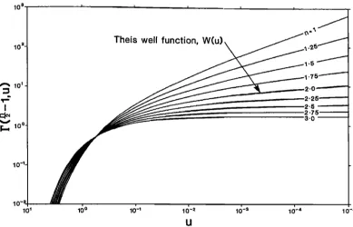
Fig. 2. Incomplete gamma function (generalized Theis well function).

10-s

where

u = Ssœr2/4Kfi

(33)

and F(a, x) is the (complementary) incomplete gamma func- tion which is shown in Figure 2.

Equation (32) is a generalization of the equation given by Theis [1935] for radial flow with a line source. An even more

general form of (32) was derived by $hchetkachev [1971] for

the case of a pumping rate which is proportional to t raised to an integral power (but only for integral dimensions). Using the

special cases of the gamma function given in (A24)-(A26) gives

e-"

h(r,

,)=

2v/;Kœb2

(•uu-

x//'•

erfc .=1 (34a)

Qo

h(r, t) = • E •(u) n = 2 (34b)

4•Ktb

h(r,

t)= Qo erfc

x//• n = 3

(34c)

4rrK fr

in which erfc is the complimentary error function and Ex is the exponential integral. Equation (34b) is the Theis equation, which is almost invariably written using the notation W(u) instead of the exponential integral. Equation (34a) was derived

by Miller [1962].

In Figure

2, which

is

a l'og-log

plot,

it appears

that

many

of

the curves tend to straight lines as u tends to zero (time tends to infinity). This behavior can be investigated by considering

the asymptotic form of (32) which, using (A22), gives

4rr-"k.rb-"v

L\Tff]

- F(1

- ,')r

2'

v :/= 0 (n • 2)

which

can be regarded

as a generalization

of the Jacob

equa-

tion [Cooper and Jacob, 1946].

Note that in (35) the time-dependent term dominates for large times when n is less than two; this explains the linear behavior in Figure 2 and also shows that the slopes of the lines tend to v (= 1 - n/2). Also, note that when v < 0 (n > 2) the time-dependent term tends to zero; hence the steady state will be achieved when and only when the dimension is greater

than two.

The integral dimension cases of (35) are

((

h(r,

t)= 2'K'zb

2 •,k,•zSsœr•,

)

--

1) n

= 1 (36a)

h(r,t)=4rcKœb

In 7-7 --7

k,S,r-J

Qo

( r( Ssf'•

"2)

h(r,

t) = 4xKj,

r 1 - k,•rKœtJ

where 3' is Euler's constant. Equation (36b) is the Jacob equa- tion and is obtained from (35) using (A18) and

lim (a • - b•)/g = In a/b (37)

3.2. I•!finitesirnal Source With a Fixed Head Boundary The case now considered is that of an infinitesimal source with a fixed head h o, boundary condition at a finite radius r o.

This case is of interest because, for the two-dimensional case,

it must leads to the Thiem equation in the steady state, and

also because it can be used for comparison with various types of numerical model, where it is easier to simulate a finite rather than infinite system.

Using the limiting form of (6), the boundary condition at

the source:

n n-t •li/•r(r,,., p) 138)

Qo/P

= - lira K fb 3-

1800 BARKER' HYDRAULIC TESTS IN ROCK

becomes

]•(r,

p) = ho/p

- Qor"[2

• -vrc-vb3

-nK

fp•V]

- 1

. (Kv(2ro)I,,(3'r)

- lv(2ro)Kv(2r)

•

•,

•I,.(-•.r

o)

7 • • (v•)•']

(39)

where use has been made of (A4), (AS), (A8), (A9), (A13), (A17), and (A34).

The steady state head distribution in this case can be ob-

tained either from the asymptotic behavior of (39) or, more

readily,

by putting

zero specific

storage

in (5) and applying

the

QoF(1

- v)

_

h(r)

-- h

o

= 4•

• _VK

fb3_nv

(r02v v • 0 (40)

which is the generalization of the Thiem equation. It can also be regarded as a special case of the generalization of Darcy's law, described by Narasimhan [1985]. Equation (40)might

have been inferred directly from (35). The specific cases of interest are

h(r)-h

o- Qo (r

o-r) n=l

(41a)

2Kib

2

Qo ln-

n=2

(4lb)

h(r)

- h

o

- 2•Kib r

- n = 3 (41c)

4•Ki

Equation (4lb), obtained by applying (37), is the Thiem equa- tion [Thiem, 19063; it is sometimes referred to as the Dupuit

formula.

3.3. Finite Source in an infinite Domain

Considering the more general case of section 3.1 where the

source has a finite radius, it is only necessary to substitute the

Laplace transform of the injection rate (29), into (21) and (25) to obtain the solution. Extension to dual-porosity media (sec-

tion 2.4) gives generalizations of the solutions presented by Moench [1984] and Barker [1985a'1, which were themselves generalizations of previous results.

As time tends to infinity, the head in the fractures tends to

that given by the generalized Theis equation (and subsequent-

ly, the Jacob equation) given in section 3.1. From (7) and (35) the head in the source is therefore related to the asymptotic fracture head by

H(t) -- (1 - 2vsf)h(r•,

t)

v < 0

(42)

head in the source H(oo) is given by

QoF(1

- v)(1

- 2vsœ)

n > 2

(43)

H(oo)

=

4rr•

_VKœb3_.

The only special case of interest is that for spherical flow'

H(

c•

) = (! + s.r)Qo

n = 3

(44)

4•r•K f

which could readily be derived from Darcy's law and (7).

4. CONSTANT HE^D TESTS

Suppose that the head in the source is held at a constant value H 0 for all times greater than zero. Using (A28), the

Laplace transform of H(t)is given by

H(p) = Ho/p

(45)

which can be used in (21) and (25) to give the injection rate

(required

to maintain

this head)

and the fracture

system

head,

source head to injection rate ratio is given by (43). For dirnen. sions less than two the injection rate tends asymptotically to

zero, while the head in the fractures (at any finite radius) tends

to that of the source.

5. SLUG TESTS

Slug tests (sometimes referred to as a pulse tests) are initiat-

ed by a sudden change of head Hi, in the source zone: a

variety of method are employed to bring about this change.

Since the storage capacity of the source is S•,, for unit change

in head, these tests can always be regarded as starting with an injection (or abstraction) of a volume S•,H• of water. Assuming this process to be effectively instantaneous, the effective injec-

tion rate is therefore

Q(t) = SwHitS(t) (46)

The Dirac delta function rS(t) has a Laplace transform of unity,

and this can be used in (21) to give the head in the source as

l•(p)

= S•,mi/{pm•,

q-

K fb3-no•nrwn-

2rl)v(kt)/[1

q-

sf(]Dv(bt)]

}

(47)

which when inverted numerically will give the slug test re-

sponse curves. (The equation for the head in the fractures is

readily obtained, but is normally of little interest.)

For large values of p (which correspond to small values of

the dimensionless

time Kœt/S•fr•,,

2) and zero skin factor,

(47}

t•(p)

= Hi/(p

+ •x•)

(48)

where

fi = b 3 -n •.r w (S•sK n- 1 s) /S•, 1/2 (49)

Equation (48) can be inverted analytically, using (A31), to give

H(t)

= H•e

• erfc

(flx•)

(50)

which generalizes a previously known result for the two- dimensional limiting case [Bredehoeft and Papadopulos, 1980]. Incidentally, (50) can be used to show that the dimensionless slope, d(H/H•)/d In t, of a slug test curve, at any given recovery

level, is independent

of the dimension

in this asymptotic

region.

Therefore

it should

be expected

that the analysis

of

slug

test

data would

often

fail to produce

a unique

dimension.

6. SINUSOIDAL TESTS

A sinusoidal

test

[Black

and

Kipp,

1981]

can

be performed

using

either

a controlled

injection

rate

or a controlled

head

in

the source. The Laplace transforms of these boundary con-

ditions

are immediately

given

by (A30),

and they

can

then

be

substituted

into (21),

(23),

or (25) to give

the required

Laplace

transform

solution

(which

can then

be inverted

numerically

to

derive the transient response).

In practice

it is normally

found

that the observed

fracture

heads

tend

rapidly

toward

steady

state

conditions

(constant

amplitude

and

phase

shift).

Therefore

for the

purposes

of

data

analysis,

only

steady

state

solutions

are

required.

Such

solu-

BARKER.: HYDRAULIC TESTS IN ROCK 1801

Fig. 3. Hypothetical fractured medium with channels.

ior of the transient solutions just described; however, a sim- pler approach to obtaining the same results will be outlined.

Assuming purely periodic behavior throughout the system:

h(r, t) = h,o(rY 'ø' (5 Z)

H(t) = H,oe i•'t (52)

Q(t) = Q,oe iø't (53)

where h,o, H,o, and Q,o are independent of t; in general, they are complex which allows the modulus of each to represent amplitude while the argument represents phase shift.

When (51) to (53) are substituted into the basic flow equa- tions (5), (6), and (7), and the exponential terms cancelled; the

resulting equations are identical to the Laplace transforms of

(5}-(7) provided:

p = i(o (54)

fi(r, p) = h,o(r) (55)

t•(p) --= H,o (56)

Q(p) • Q,o (57)

Therefore (21), (23), and (25) can be used directly to give

steady state sinusoidal solutions. For example, for a controlled

sinusoidal injection rate, (2,ø can be set equal to the amplitude of the injection rate (no phase shift), and (54), (55), and (57) can be used in (25) to give an equation for h,•, the response of the

fracture system. If this result is simplified by setting the skin factor to zero and the dimension to two, the result given by Black and Kipp [1981] is obtained.

7. DISCUSSION

7.1. Application to Fractured Rock

There are two reasons for proposing the GRF model as a

candidate for use in simulating hydraulic tests in fractured

rock. First, it contains few parameters yet permits a great

range of behavior patterns; this makes it particularly suitable for data analysis. Second, since the dimension of the flow

system is difficult to choose, it is a natural choice for gener-

alization. Even if it were to be demonstrated that the flow dimension must assume integral values, the GRF model is still of value in that it provides a single formulation for all three dimensions. There is no intention to suggest that this model

should

replace

existing

models,

some

of which

have special

characteristics [e.g., Hsieh, 1983: Karasaki, 1986] which makes them a more obvious choice under certain circum-

stances.

7.2. Parameters

The GRF model introduces two novel parameters: the di- mension n and the extent of the flow zone b. Tortuosity is also

introduced, but is used in the familiar sense to represent the ratio of the length of the flow path between two points and the

distance between the same points.

The parameter b is difficult to describe for nonintegral flow dimensions, but it has a simple interpretation for integral values. For one-dimensional flow it is simply the square root

of the flow area (Figure la). For two-dimensional flow b is the extent of the flow region perpendicular to the plane of flow

(for example, the thickness of a confined aquifer, Figure lb). For spherical flow the parameter has no significance: this is possible mathematically because b appears raised to the power of 3- n in the flow equations, so this term reduces to unity

when n = 3.

While it is natural to characterize the hydrogeological properties of rock by its hydraulic conductivity and specific storage, the general solution given by (21), (23), and (25) sug-

gests

the use

of the

diffusivity

K•,/Ss•,

and

the quantity

b3-nKf

(which becomes the transmissivity in the two-dimensional case). Indeed, to extract any two of the parameters contained in these groups (not counting the dimension n which appears independently in the equations) the third must be known a priori.

The meaning of the dimension n in the case of nonintegral values is probably the most difficult conceptual feature of the model. This value may only be meaningful within the context of more fundamental models. For example, it might be ex- pected that the dimension would be related to a characteristic statistical property of a fracture network model. (Work on investigating such a relationship has already begun). A reason- able conjecture would be that radial diffusion (Brownian motion) on a fractal network of dimension n would be de- scribed by (5). And these two ideas are related through the observation that real fracture networks appear to have fracta! properties [e.g., Long et al., 1985].

The dimension does not appear to be an intrinsic hydraulic

property of the fracture system, which is obviously an unsatis- factory feature of the model. Consider the hypothetical system depicted in Figure 3, where water flows in an infinite system of

channels within a plane. Imagine a test where water is injected

at point A, the pressure response at point B might reasonably be expected to be (approximately) characteristic of flow in a

linear system, at least for early times. However, for a long- term test, the pressure response at point C (and possibly also

at point B) would be more likely to be characteristic of cylin-

drical flow. This scale dependence of the dimension is some-

what analogous to that of the dispersion coefficient used in transport modeling, which, nevertheless, has proved to be a

useful parameter.

The dimension is not related to any angular restriction on the flow direction. For example, steady state flow within a

cone from a point source at its apex would be truly spherical

flow (n = 3).

The dimension is not related to the space-filling character-

istics of the flow paths. For example, a spiral flow channel

1802 BARKER:HYDRAULIC TESTS IN Roc•

sufficient)

that for flow systems

to have different

dimensions

7.3. Anisotropy

The GRF model does not appear to permit the introduction

of anisotropy

in cases

of nonintegral

dimerOsion

(since

a con-

ductivity

tensor

must

have an integral

number

of terms).

Be-

cause of the tendency of rocks to fracture along particular

directions,

a homogeneous

model

with anisotropy

[e.g.,

Hsieh,

1983]

will often

be more

valid

than the GRF model,

particu-

7.4. Finite Source

Several solutions have been given which relate to an ideal n-dimensional spherical source (notably the slug test solution).

In practice,

such

a source

cannot

be realized

except

for inte-

gral dimensions.

So the head in a real source

cannot

be ex-

pected

to correspond

closely

to the value of H, although

it

could be hoped that variations in H might be indicative of real head changes. Because of this difficulty the model is more applicable to interference tests than to single borehole tests.

7.5. Sinusoidal Tests

Although the GRF model was originally developed for the analysis of data from sinusoidal tests, there are special difficul- ties in applying it to such tests. A single test results in only two numbers (a phase shift and an amplitude)so several tests are required to obtain a complete set of model parameters.

Further information can be obtained by varying the frequency of the test [Black et aI., 1986]; however, the derived dimension

is likely to decrease with increasing frequency, since the radius

of influence of the test will decrease. Tests over various dis- tances can also be used, but again the problem of dimension

varying with scale arises.

7.6. Relationship to Other Models

The main reason for carrying out hydraulic tests is usually to obtain parameter values that can be used in some form of

regional flow model. If the GRF model reveals an integral dimension for a test then the only problem is that of deciding

the orientation of the flow system when the dimension is either

one or two. However, for nonintegra! dimensions the model, along with any parameters derived using it, is not consistent

with any commonly used model. It is hoped, however, that it will be possible to establish a relationship between the GRF

model and fracture network models.

8. CONCLUSIONS

Mathematical solutions have been derived for the common-

ly used forms of hydraulic test for an arbitrary flow dimension.

These solutions include generalizations of many well-known formulae used for pumping test analysis, including the Theis

equation, (32), the Jacob equation, (35), and the Thiem equa-

tion (40).

The more general solutions are expressed in terms of the

Laplace transforms of the time-dependent heads and injection rate. The solutions include well bore skin and, in section 2.4, it

is shown that these are easily extended to include dual poros-

ity. Normally, it will be necessary to invert these transforms

numerically; a brief discussion of methods is given in Appen-

dix B.

Constant rate tests in an infinite medium will tend to a

steady state for all dimensions greater than two. Steady state solutions are diagnostic of the dimension via the radial vari- ation in head. When the dimension is less than or equal to two, the test will be transient; when it is less than two, the dimension is obtained directly from the slope of a plot of the

logarithm

of head against

the logarithm

of time, for large

The model is a straightforward extension of integral dimcu.

sion models and it therefore appears to be a natural candidate for a model of flow in fractured rock, where the appropriate dimension is often uncertain. However, significant theoretical

and practical difficulties arise in the application of the model.,

notably, the dimension does not appear to be an intrinsic

property of the rock (and is likely to be scale-dependent), the

idealized spherical source geometry cannot be realized, and

anisotropy cannot be included. Also, the physical interpreta. tion of the flow dimension is unclear, although it is conjec-

tured that the model respresents radial diffusion on a fractal network. Numerical experiments using fracture network models should help to give some insight into these problems.

APPENDIX A: MATHEMATICAL FORMULAE

This appendix provides a set of useful mathematical formu-

lae which have been drawn from various sources, often with some modification. Most are employed within the derivations

in this paper, but others will be of value either in simplifying the formulae in special cases or in evaluating the results.

Unless otherwise stated: the symbols z and 2 represent com- plex numbers, v, a, and n are real (possibly integer) numbers, and N is an integer.

Modified Bessel Function of the First Kind: Iv(z )

Iv(z

) = e-(•/2)v•iJv(ze(•/2)•i

)

--re

< arg z < «re

(AI} = e(3/2)v'aJv(ze-(3/2)•i ) «• < arg z _< re

Iv - x

(z) -- I v + x

(z) -- 2vlv(z)/z

(A2}

I _ N(z)

= IN(z)

(A3)

lim z-Vlv(z)

= 2-v/F(1

+ v)

v • --1, --2, ...

(A4)

z--•0

d z•lv(2z)

,tz•I•_

x(,;tz)

(A5)

dz

Macdonald (Bessel) Function' K,(z)

Kv(z

) =• [I_•(z)-

Iv(z)]/sin

(v•r)

(A6}

K•(z)

= lim K•(z)

(A7}

.

K_•(z)

= Kv(z)

lira

z•K•(z)=

2•- xF(v) v > 0

Z'-*0

lim

[z-•Kv(z)-

2•- xF(v)z

-2v]

= --2-•-xF(

1 -- v)/v {AI0}

v -• integer

v>O

D

(All)

lim

•vv

K•(z)

= 0

v-'*0

(2-•-)

t/2

BARKER' HYDRAULIC TES'rS IN ROCK I803

d/dr ,., Kv(,,.z) -- -zz K•_ •(2z) (A13)

= e--' (A14)

K 3/2(z) = (1 + 1/z)e -: (A 15) Gamma Function' F(v)

F(1 + v) = vF(v) (A 16)

F(v)F(1 -- v) = • csc (•v) (A17) In F(1 - x)

lim = 7 (A18)

x•O X

r(• • •

(A

19)

F(•) • • (A20)

r(•) • •

(A21)

Incompteee Gamma Function' F(a, x)

F(a,x)

F(a)

• (--1)•x

•*•

(A22) (A23) (A24) (A25) (A26)

OF(a, x)/Ox = - x a- • e- x r(0, x)= Z(x)

F(«,

x)= x//-•

erfc

F(-«, x): 2(e-X/x//•-

• erfc

•)

Laplace Transforms

©

L{f(t)} =•½)= e-r7(t) dt (A27)

L{ 1 ) = 1/r (A28)

L{•(t)} = 1 (A29)

L{sin wt} = o/(w 2 + p2) (A30)

{a)3 =

+

L • • F -v, • p-t•/2>-•K,.(a•)

(A32)

lim pL{f(t)} = lim f(t) (A33)

p•O t•

Unit Sphere in n Dimensions

area = % = 2•"/2/F(n/2) (A34)

volume = •/2/F(1 + n/2) (A35)

See also Table 1.

APPENDIX B: EVALUATION OF FORMULAE

Many of the results given in this paper are expressed in the

form

of Laplace

transforms

of the time-dependent

functions

of

sary to invert the transform. Analytical inversion is generally impractical so numerical inversion must be employed. Even if

analytical

inversion

were possible,

the resulting

formulae

would

normally

be so complex

that they

would

be more

diffi-

cult

and computationally

expensive

to evaluate

directly

than

by numerical inversion of their transforms.

The most

commonly

used

Laplace

transform

inversion

al-

gorithm is that given by Stehfest [1970]; however, the author has found the method described by Talbot [1979] to be su-

perior both in terms of' speed and accuracy.

To employ the Talbot algorithm the transform function must be expressed in terms oœ a complex transform variable p, and this requires the evaluation of' Bessel functions of complex

argument. These complex functions are also required to evalu-

ate the sinusoidal solutions described in section 6 even though no transform inversion is involved. The CERN Subroutine Library [Strassen, 1975] provides a routine for the evaluation of d,.(z), and using (A1), (A6), and (A7) this can provide rou- tines adequate for evaluating all of the formulae given in this paper. However, a recently developed package of routines

[Amos, 1986] provides a more accurate and efficient set of functions and is strongly recommended.

NOTATION

a volume to area ratio for a matrix block.

b extent of the flow region (e.g., Figure 1).

B(•) block geometry function for dual-porosity media. erfc (x) complementary error function.

E•(u) exponential integral (Theis well function). h(r) steady state head in fracture system. h(r, t) transient head in fracture system.

h o fixed head in fractures at radius r 0.

h,o(r) (complex) head in fractures due to a sinusoidal

source.

H(t) head in source.

H• initial head in source during a slug test. H o source head during a constant head test. H,o (complex) source head during a sinusoidal test.

i

Iv(z ) modified Bessel function.

Jr(z) Bessel function.

K•- hydraulic conductivity of the fracture system.

K,• hydraulic conductivity of the rock matrix. K•(z) modified Bessel function.

n dimension of the fracture flow system. p Laplace transform variable.

q volumetric flow rate of water.

Q(t) volumetric rate of injection into the source. Qo volumetric rate of injection during a constant rate

test.

Q•, (complex) amplitude of the injection rate during a sinusoidal test.

r radial distance from the centre of the source (measured along the flow paths).

ro radius at which a fixed head h o is specified. % radius of the source.

sj. skin factor,

defined

by (7).

Ss• specific

storage

of the fracture

system.

Ss,, specific storage of. the rock matrix.

Sw storage capacity of the source. t time.

u---

Ssfr2/4Kft.

W(u) Theis well function.

% area of a unit sphere in n dimensions. fi see (49).

•, Euler's constant (-0.5772...).

F(x) gamma function.

1804 BARKER: HYDRAULIC TESTS IN ROC}t

cS(t) Dirac delta function.

2---(pSsf/Kf)

•/2 (see

also

equation

(26)).

/• = ,•.r •,. v = 1 -- n/2. • =(PSsma2/Km) •/2

a ratio of matrix storage to fracture storage per

unit volume.

½v(z) = zK v_ ,(z)/K,,(z).

o• angular frequency for a sinusoidal test.

AcknowledFments. This work was motivated by the hydraulic test- ing programme carried out in the Stripa mine, and I would like to acknowledge the work of my colleagues on that programme; dis- cussions with John Black and David Noy were particularly stimu- lating. Brief discussions with Jane Long and Kenzi Karasaki (Law- rence Berkeley Laboratory) were a valuable source of encouragement. The comments of the referees were also appreciated. This paper is published with the approval of the Director, British Geological

Survey (NERC).

REFERENCES

Amos, D. E., Algorithm 664: A portable package for Bessel functions of a complex argument and nonnegative order, ACM Trans. Math. Software, I2(3), 265-273, 1986.

Barker, J. A., Generalized well-function evaluation for homogeneous and fissured aquifers, J. Hydrol., 76, 143-154, 1985a.

Barker, J. A., Block-geometry functions characterizing transport in densely fissured media, .1. Hydrol., 77, 263-279, 1985b.

Barker, J. A., Modelling the effects of matrix diffusion on transport in densely fissured media, Mere. lnt. Assoc. Hydrogeol., 18, 250-269,

1985c.

Black, J. H., J. A. Barker, and D. J. Noy, Crosshole investigations: the method, theory and analysis of crosshole sinusoidal pressure tests in fissured rock, Stripa Proj., Int. Rep. 86-03, SKB, Stockholm,

1986.

Black, J. H., and K. L. Kipp, Determination of hydrogeological pa- rameters using sinusoidal tests: A theoretical appraisal, Water

Resour. Res., 17(3), 686-692, 1981.

Bredehoeft, J. D., and S.S. Papadopulos, A method for determining

the hydraulic

properties

of tight

formations,

Water

Resour.

Res.,

Cooper, H. H., Jr., and C. E. Jacob, A generalized method for evalu.

ating formation constants and summarizing well-field history, Eos

Trans. AGU, 27, 526-534, 1946.

Hsieh, P. A., Theoretical and field studies of fluid flow in fractured rocks, Ph.D. dissertation, 200 pp., Univ. of Ariz., Tucson, 1983.

Karasaki, K., Well test analysis in fractured media, Ph.D. dissertation,

239 pp., Univ. of Calif., Berkeley, 1986.

Long, J. C. S., H. K. Endo, K. Karasaki, L. Pyrak, P. MacLean, and

P. A. Witherspoon, Hydrologic behavior of fracture networks,

Mem. lnt. Assoc. Hydrogeol., 17, 449-462, 1985.

Miller, F. G., Theory of unsteady-state inflow of water in linear reset.

volts, d. Inst. Pet., 48, 467-477, 1962.

Moench, A. F., Double-porosity models for a fissured groundwater

reservoir with fracture skin, Water Resour. Res., 20(7), 831-846,

1984.

Narasimhan, T. N., Geometry-imbedded Darcy's law and transient subsurface flow, Water Resour. Res., 21(8), 1285-1292, 1985. Ramey, H. J., Jr., Well-loss function and the skin effect: A review, in

Recent Trends in Hydrogeology, edited by T. N. Narasimhan, Geo. logical Society of America, Boulder, Colo., 1982.

Shchelkachev, V. N., A general solution for the differential equations of one-dimensional nonstationary flows in a multidimensional space, News Acad. Sci. USSR: Liqud Gas Mech., 3, 481-487, 1971. Stehfest, H., Numerical inversion of Laplace transforms, Commun.

ACM, 13(1), 47-49, 1970.

Strassen, H. H., Double precision complex Bessel function Jr(z), Rou- tine C332, CERN Computer Centre Program Library, Geneva,

1975.

Talbot, A., The accurate numerical inversion of Laplace transforms, J. Inst. Math. Appl., 23, 97-120, 1979.

Theis, C. V., The relation between the lowering of the piezometric surface and the rate and duration of discharge of a well using groundwater storage, Eos Trans. AGU, 16, 519-524, 1935.

Thiem, G., Hydrologische Methoden, J. M. Gebhardt, Leipzig, 1906.

J. A. Barker, British Geological Survey, Maclean Building, Crow- marsh Gifford, Wallingford, Oxfordshire, OX10 8BB United King-

dom.

(Received February 17, 1988;

revised May 25, 1988;