Vector-Vector Scattering on the Lattice

Vector-Vector Scattering on the Lattice

FernandoRomero-López1,_{,CarstenUrbach}1_{, andAkakiRusetsky}1,

1_{HISKP (Theory) and BCTP, University of Bonn, Germany}

Abstract.In this work we present an extension of the Lüscher formalism to include the interaction of particles with spin, focusing on the scattering of two vector particles. The derived formalism will be applied to Scalar QED in the Higgs Phase, where the U(1) gauge boson acquires mass.

1 Introduction

The study of scattering in Lattice Field Theory starts with the original work of Lüscher [1]. In this first work, he derived equations for the scattering length and phase shift of spinless particles in the rest frame. The formalism has been extended to include moving frames [2],π−Nscattering [3],N−N

scattering [4], different masses [5,6], moving frames with different masses and one particle with spin 1/2 [7] and any multichannel system with arbitrary spin, momentum and masses [8].

In this work, we derive a general Lüscher equation for scattering of particles with arbitrary spin through the matching to a non-relativistic effective theory. The results obtained here are in agreement with Ref. [8]. We will focus on the case of two identical vector particles and we will make use of the spatial symmetries of the lattice to factorize the Lüscher equation. By means of operators that transform under a certain irreducible representation of the spatial symmetry group, we gain access to the different phase shifts of the theory. The equations will be tested in Scalar QED, for which first numerical results will be shown.

2 Scattering of two vector particles

2.1 Derivation of Lüscher Equation for Arbitrary Spin

Let us consider a system of two particles with masses Mi,i = 1,2 and described by the effective

non-relativistic Lagrangian:

L=φ†₁2W1(i∂t−W1)φ1+φ†₂2W2(i∂t−W2)φ2+LI. (1)

Here,φiare the non relativistic fields with spinsi andWi = (M2_i − ∇2)1/2. The corresponding

non-relativistic propagators, withωi=(M_i2+p2)1/2, read

Si(p)= 1

2ωi(p)

1

ωi(p)−p0−i, (2)

The scattering T matrix is defined through the Lippman-Schwinger (LS) equation:

T(z)=(−HI)+(−HI)(−G0(z))T(z), (3)

whereG0(z)=(z−H0)−1is the free resolvent and the two particle states coupled to a spin S are

|k1,k2,S, ν ≡ |P,k,S, ν, (4)

P_{,k,S, ν|P,k,S, ν=4ω}

1ω2(2π)dδd(P−P)(2π)dδd(k−k)δS_Sδνν, (5)

P=k₁+k₂, k=µ2k1−µ1k2, µ1,2= 1₂



1±m21_P−₂m22



, (6)

whereS,νlabel the total spin of the two particle system andP,kare the total and relative momentum in the “laboratory frame”. Now define the matrix elements:

tS_S

ν_ν(k,k,P,z)=

_dd_P

(2π)dP,k,S, ν|T(z)|P,k,S, ν, (7)

hS_S

ν_ν(k,k,P)=

_dd_P

(2π)d P,k,S, ν|(−HI)|P,k,S, ν. (8)

Additionally, G0 can be written in terms of an elementary diagram using the Feynman rules and

one can perform the integration overq0_{using the Cauchy integration formula. One may rewrite the}

Lippman-Schwinger Equation in terms of matrix elements using Equations7and8:

tS_S

ν_ν(k,k,P,z)=hS _S

ν_ν(k,k,P)+ _dd_q

1 (2π)d

ν

hS_S

ν_ν(k,q1,P)tS _S

ν_ν(q1,k,P,z)

4ω1(q1)ω2(P−q1).(ω1(q1)+ω2(P−q1)−z), (9)

whereq=µ2q1−µ1q2, as in Equation6. A key point here is that the elementary bubble is diagonal in spin, because also the single particle propagators are. However, the scattering amplitude need not be diagonal. Now define the projectors to the partial waves in the CM frame, whose momenta arek∗_:

Π_νA_νA(k∗,k∗)=

ρ,ρ

US

ν_ρ(k∗)∗US_νρ(k∗)(YJ_lSµ(k∗, ρ))∗YJlSµ(k∗, ρ), (10)

A=(J,l,S, µ), A=(J,l,S, µ), (11)

whereUS_νρ(k∗_{) is the unitary transformation of the spin indices under a boost and the spin spherical} harmonics, withˆk=k/_|k_|, read

YJlSµ(k, ν)=

m,σ

lmSσ_|Jµ _|k_|lYlm(ˆk)χSσ(ν)≡ |k|lYJlSµ(ˆk, ν). (12)

Using the projectors, Equations7and8take the form

tS_S

νν(k,k,P,z)=4π

A,A

ΠA_ννA(k∗,k∗)tAA(s,P,z), (13)

hS_S

νν(k,k,P)=4π

A_,A

ΠA_ννA(k∗,k∗)hAA(s,P). (14)

If the system is placed in a box, the integral may be replaced by an sum: _dd_q

1 (2π)d →

1

L3

q1

The scattering T matrix is defined through the Lippman-Schwinger (LS) equation:

T(z)=(−HI)+(−HI)(−G0(z))T(z), (3)

whereG0(z)=(z−H0)−1is the free resolvent and the two particle states coupled to a spin S are

|k1,k2,S, ν ≡ |P,k,S, ν, (4)

P_{,k,S, ν|P,k,S, ν=4ω}

1ω2(2π)dδd(P−P)(2π)dδd(k−k)δS_Sδνν, (5)

P=k₁+k₂, k=µ2k1−µ1k2, µ1,2= 1₂



1±m21_P−₂m22



, (6)

whereS,νlabel the total spin of the two particle system andP,kare the total and relative momentum in the “laboratory frame”. Now define the matrix elements:

tS_S

ν_ν(k,k,P,z)=

_dd_P

(2π)dP,k,S, ν|T(z)|P,k,S, ν, (7)

hS_S

ν_ν(k,k,P)=

_dd_P

(2π)d P,k,S, ν|(−HI)|P,k,S, ν. (8)

Additionally, G0 can be written in terms of an elementary diagram using the Feynman rules and

one can perform the integration overq0_{using the Cauchy integration formula. One may rewrite the}

Lippman-Schwinger Equation in terms of matrix elements using Equations7and8:

tS_S

ν_ν(k,k,P,z)=hS _S

ν_ν(k,k,P)+ _dd_q

1 (2π)d

ν

hS_S

ν_ν(k,q1,P)tS _S

ν_ν(q1,k,P,z)

4ω1(q1)ω2(P−q1).(ω1(q1)+ω2(P−q1)−z), (9)

whereq=µ2q1−µ1q2, as in Equation6. A key point here is that the elementary bubble is diagonal in spin, because also the single particle propagators are. However, the scattering amplitude need not be diagonal. Now define the projectors to the partial waves in the CM frame, whose momenta arek∗_:

ΠA_ννA(k∗,k∗)=

ρ,ρ

US

ν_ρ(k∗)∗U_νρS(k∗)(YJ_lSµ(k∗, ρ))∗YJlSµ(k∗, ρ), (10)

A=(J,l,S, µ), A=(J,l,S, µ), (11)

whereU_νρ(S _k∗_{) is the unitary transformation of the spin indices under a boost and the spin spherical} harmonics, withˆk=k/_|k_|, read

YJlSµ(k, ν)=

m,σ

lmSσ_|Jµ _|k_|lYlm(ˆk)χSσ(ν)≡ |k|lYJlSµ(ˆk, ν). (12)

Using the projectors, Equations7and8take the form

tS_S

νν(k,k,P,z)=4π

A,A

ΠA_ννA(k∗,k∗)tAA(s,P,z), (13)

hS_S

νν(k,k,P)=4π

A_,A

ΠA_ννA(k∗,k∗)hAA(s,P). (14)

If the system is placed in a box, the integral may be replaced by an sum: _dd_q

1 (2π)d →

1

L3

q1

, (15)

and by plugging Equations13and14into Equation9on the mass-shell, one arrives to

tA_A(s,P)−h_AA(s,P)= k ∗

8π√s

B,B

hA_B(s,P)((k∗)l+lil−lδ_SBSBMBB(s,P))t_BA(s,P), (16)

withs=P2andSBbeing the spin of the multi-indexBas in Equation11. Now, using unitarity of the

transformation of the spin indices, one arrives at

MJlSµ,J_lSµ(s,P)= 32π

2

k∗

√_s

L3i l_−l

δS_S

q1

_ν(Y

JlSµ(ˆq∗, ν))∗YJ_lSµ(ˆq∗, ν)

4ω1(q1)ω2(P−q1)(ω1(q1)+ω2(P−q1)−P0). (17)

This matrix can be related to its equivalent for scalar particles by using Equation12:

MJlSµ,JlSµ=δSS

m,m_,σ

lm,Sσ_|Jµ l_{m,Sσ|Jµ Mlm}

,lm, (18)

where we used the identity [5,9] (withq=q₁₋µ1P)

1

4ω1ω2(ω1+ω2−P0)

= 1 2P0

1 q2₋(qP)2 P2

0 −(k

∗₎2

+ 1 4ω1ω2

1

ω1+ω2+P0 −

1

ω1−ω2+P0 −

1 ω2−ω1+P0

, (19)

kept only the divergent part (first term in Equation19) and used (q∗₎2_=q2₋(qP)2 P2

0 . This way, and up

to exponentially suppressed terms (q∗_→k∗_),Mlm

,lmis given by (see [5])

Mlm,lm(k∗,s)= (−1)

l

π3/2_γ l+l

j=|l−l_|

j

s=−j

ij

ηj+1Z

d

js(1,s)∗Clm,js,lm, η=|k ∗_|L

2π , (20)

where

Clm,js,l_m=(−1)mil−j+l(2l+1)(2l+1)(2j+1)

l j l

m s −m l j l 0 0 0

, (21)

Zd lm(1,s)=

r∈Pd

|r|lYlm(r)

r2_−η2 , Pd ={r||=γ−1(n||−µ1d),r⊥=n⊥}, (22)

withn∈Z. One can see that Equation16is a matrix equation, and the poles intA_Aarise when

det

8π√s

(k∗₎l+l+1(h

J

lS,l_S)−1δJJδµµ−δS,SMJlSµ,JlSµ

=0, (23)

where it is already implied thatJandµare conserved in scattering processes in infinite volume and mixings can be present inlandS,hJlSµ,J_lSµ =h_lSJ_,lSδ_JJδµµ. In order to express this equation in a more compact way, one uses the standard definition of theS matrix (see [10], for nucleon-nucleon scattering),S =e2iδ(s), in terms of the phase shiftδ(s). This way, one can expresshJ_lS,lSin terms ofδ:

hJ lS,l_S =

8π√s

(k∗₎l+l+1(tanδ)

J

lS,l_S, (24)

and plugging it in Equation23, we arrive at

det(cotδ)J

lS,l_SδJJδµµ−δS SMJlSµ,JlSµ

2.2 Two Vector Particles

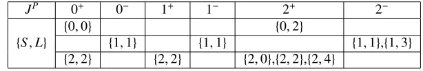
A system of two identical vector particles can couple to total spinS =0,1,2. Even spin combinations are symmetric under the exchange of two particles, whereas odd combinations are antisymmetric. The same holds for the angular momentumL. The possible combinations ofS andLtoJP_{respecting the}

Bose statistics (totally symmetric state) are listed in the Table1. The combinations that have mixing are in the same column in the table and correspond to sameJP_{but differentL,S.}

JP ₀+ ₀− ₁+ ₁− ₂+ ₂−

{S,L} {

0,0} {0,2}

{1,1} {1,1} {1,1},{1,3}

{2,2} {2,2} {2,0},{2,2},{2,4}

Table 1.Possible values ofJP_withJ<3.

The possible mixings can be parametrized with a mixing angle and two eigenvalues. This would be analogous to the parametrization of the mixings for two nucleons in Reference [10].

For the scattering of two spinless particles, it is well known that the phase shift can be parametrized as a polynomial ofk2_{. Such an equivalent parametrization can be derived here as well:}

kl+l+1_cotδJ

lS,l_S=

n=0

ank2n. (26)

2.3 Reduction of Lüscher Equation

The basis vector labeled byαof a symmetry groupG, in a certain irreducible representationΓ, are constructed (up to normalization) applying the projector

(PΓ,J,l

αβ )µµ=

i∈G

(RΓ

i)∗αβD˜Jµµ,l(Ri), (27)

to the basis vectors in the continuum,|J,S,l, µ, for a fixedβandµ:

|Γ, α,J,S,l,n ∝

µ (PΓ,J,l

αβ )µµ|J,S,l, µ, (28)

where n labels the number of occurrences of Γ in J, l. In the previous equations ˜D_µµJ,l(Ri) =

(−1)l_DJ

µµ(Ri) if the elementiincludes inversion, or just the standard Wigner matrix if not. The basis vectors of the irreducible representations of the symmetry group of the lattice can be expressed in terms of the one of the continuum:

|Γ, α,J,l,S,n= µ

cΓnα

Jlµ |JlSµ, (29)

where the coefficients cΓnα

Jlµ are to be read from basis vector tables in References [7] and [3], for example. The matrixMcan be partially diagonalized in this basis:

Γ, α,J_{,l,S,n|M|Γ, α,J,l,S,n=M}Γ

J_{lS n,JlS n}δΓΓδαα, (30)

MΓ

J_{lS n,JlS n}=

µµ (cΓn_α

2.2 Two Vector Particles

A system of two identical vector particles can couple to total spinS =0,1,2. Even spin combinations are symmetric under the exchange of two particles, whereas odd combinations are antisymmetric. The same holds for the angular momentumL. The possible combinations ofS andLtoJP_{respecting the}

Bose statistics (totally symmetric state) are listed in the Table1. The combinations that have mixing are in the same column in the table and correspond to sameJP_{but differentL,S.}

JP ₀+ ₀− ₁+ ₁− ₂+ ₂−

{S,L} {

0,0} {0,2}

{1,1} {1,1} {1,1},{1,3}

{2,2} {2,2} {2,0},{2,2},{2,4}

Table 1.Possible values ofJP_withJ<3.

The possible mixings can be parametrized with a mixing angle and two eigenvalues. This would be analogous to the parametrization of the mixings for two nucleons in Reference [10].

For the scattering of two spinless particles, it is well known that the phase shift can be parametrized as a polynomial ofk2_{. Such an equivalent parametrization can be derived here as well:}

kl+l+1_cotδJ

lS,l_S=

n=0

ank2n. (26)

2.3 Reduction of Lüscher Equation

The basis vector labeled byαof a symmetry groupG, in a certain irreducible representationΓ, are constructed (up to normalization) applying the projector

(PΓ,J,l

αβ )µµ =

i∈G

(RΓ

i)∗αβD˜µµJ,l(Ri), (27)

to the basis vectors in the continuum,|J,S,l, µ, for a fixedβandµ:

|Γ, α,J,S,l,n ∝

µ (PΓ,J,l

αβ )µµ|J,S,l, µ, (28)

where n labels the number of occurrences of Γ in J, l. In the previous equations ˜D_µµJ,l(Ri) =

(−1)l_DJ

µµ(Ri) if the elementiincludes inversion, or just the standard Wigner matrix if not. The basis vectors of the irreducible representations of the symmetry group of the lattice can be expressed in terms of the one of the continuum:

|Γ, α,J,l,S,n= µ

cΓnα

Jlµ |JlSµ, (29)

where the coefficients cΓnα

Jlµ are to be read from basis vector tables in References [7] and [3], for example. The matrixMcan be partially diagonalized in this basis:

Γ, α,J_{,l,S,n|M|Γ, α,J,l,S,n=M}Γ

J_{lS n,JlS n}δΓΓδαα, (30)

MΓ

J_{lS n,JlS n}=

µµ (cΓn_α

J_lµ)∗c_JlΓn_µαMJ_lSµ,JlSµ. (31)

Moreover, the matrix cotδhas to be brought to the same basis asM:

(cotδ)Γ

JlS n,J_lSn=

µµ (cΓn_α

J_lµ)∗cΓ_Jln_µα(cotδ)_lSJ_,lSδµµδ_JJ=

µ (cΓn_α

Jl_µ)∗cΓ_Jln_µα(cotδ)_lSJ_,lSδJJ. (32)

The coefficientscΓnα

Jlµ just depend on the total angular momentum Jand the behaviour under spatial inversions (−1)l_{. Moreover, mixing can only occur between states with sameJand (−1)}l_{, so the sum}

over the indexµyields either 1 or the matrix cotδis trivially zero due to the symmetry considerations. Spin does not enter here at all, because it does not influence the coefficients. This way, (cotδ)Γ

JlS n,JlSn is diagonal inJandnand the determinant factorizes:

S=e_oddven

Γ

det(cotδ)J

lS,l_SδJJδ_nn−δ_{S S}MΓ_{JlS n,JlS n}

=0. (33)

3 Toy Model: Scalar QED

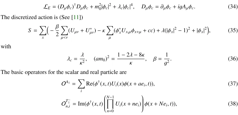
In order to test the formalism, we use Scalar QED with a Higgs mechanism, since the vector state needs to be massive. The continuum Euclidean Lagrangian of such a theory reads

LE =(Dµφc)†Dµφc+m20|φc|2+λc|φc|4, Dµφc=∂µφc+igAµφc. (34)

The discretized action is (See [11])

S =

x

−β₂

µ<ν

(Uµν+Uµν)∗ −κ

µ (φ∗

xUx,µφx+µ+cc)+λ(|φx|2−1)2+|φx|2

, (35)

with

λc= λ

κ2, (am0)

2₌1−2λ−8κ

κ , β=

1

g2. (36)

The basic operators for the scalar and real particle are

OA1₌ i

Re(φ†_(x,t)U

i(x)φ(x+aei,t)), (37)

OT1−

n,i =Im(φ†(x,t)

  

N−1

n=0

Ui(x+nei)

 

φ(x+Nei,t)), (38)

respectively. Notice that the second one is highly non-local, since this have been seen to improve significantly the signal. In particular, with the vector operator, one can build one and two particle operators that transform under certain irreducible representations of the spatial symmetry group, in rest and moving frames. A one particle operator transforming under a certain irrepΓwith invariant momentum under the spacial symmetry groupp∈ Gcan be built from an arbitrary operatorO(x,t) as follows:

OΓ_(p,t)=

x

eipx Si∈G

χΓ_(S

i) (SiO)(Si−1x,t) (39)

Equivalently, for a two particle operator:

OΓ_(p,q,t)=

x,y   

Si∈G

eipx+Siq(y−x)

  

Si∈G

χΓ_(S

i) (SiO)(S−i1x,S−i1y,t), (40)

4 Numerical Results

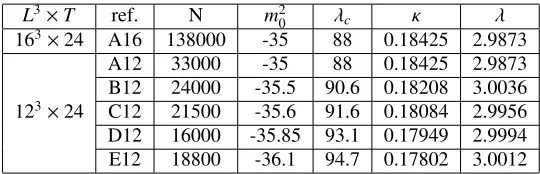
We use five different parameters forL=12 and for one parameter setL =12 andL=16 (see Table

2). In Figure1(a)we show the dependence of mass of the vector particle on the length of the operator in Equation38for ensemble A12. The results show a clear improvement of the signal with non-local operators. When using moving frames, the best signal is empirically seen atN =L/(d+1), beingd the units of momentum in that particular direction.

Moreover, we study the mass of a single vector and scalar particle in theL =12 volume for the different bare parameter sets (Figure1(b)). In the continuum, the bare masses of the particles are

m2

φ =−2m20andm2V =−

g2m2 0

λc . The mass of the vector is suppressed bygandλc, and it seems logical

that it is much smaller than the scalar mass. However, it is not clear why the scalar mass duplicates with increasingκ, whereas the vector mass increases slightly. Naïvely, the increase of the vector mass should be enhanced by the reduction ofλcwith increasingκ, but there seems to be some non-trivial

behaviour.

The energy difference∆Eis defined as the difference between the two particle energy on the lattice and the two particle energy in absence of interactions. In Figure1(c)we show the results for∆Eas a function ofκ. For higherκ, the interaction generates scattering states (∆E >0) with2σstatistical significance. Asκbecomes smaller, all particles become lighter and the interaction seems to flip sign. For the lowest values ofκ, the two particle states are bound states (∆E<0), with a similar statistical significance as in the other case. Unfortunately, in the transition region the statistical significance is rather small. Besides, we see the expected volume dependence in the energy shift, when comparing

L=12 withL=16.

In addition, we show the results of the mass of a single vector particle for the different irreps in Figure1(d). The values for the different moving frames tend to always larger than the one in the rest frame. Since the correlation functions are fitted to include an excited state, a contamination of higher states is likely not the main reason. It is however true that from the correlation functions one obtains upper bounds for the energy, which might have an influence. In addition, the different irreps seem to split. In particularA1andEseem to differ by around 3σ.

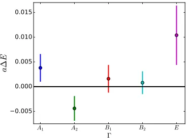
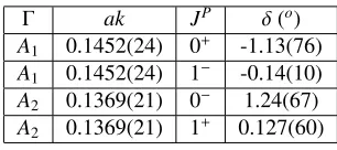
Furthermore, in Figure1(e)we show∆Efor the ensemble A16 in the first moving frame. One can see how the different irreps split. With these values one can calculate phase shifts values (Table

3). Finally, in Figure1(f)we show all our results for the phase shift with JP _{= 0}+_{. For the highest}

momentum shown, the ratio between the non-relativistic kinetic energy and the mass is quite large,

Ek

m ≈ 0.8. Hence, the kinematic suppression of higher partial waves, though present, is not strong

any more and a corresponding systematical error is to be expected. Still, it seems that the phase shift increases for the last points. If this increase is physical, it could correspond to a resonance around scattering momentumak≈0.18.

L3_{×T ref. N m}2

0 λc κ λ

163_{×24 A16 138000 -35 88 0.18425 2.9873}

123_×24

A12 33000 -35 88 0.18425 2.9873 B12 24000 -35.5 90.6 0.18208 3.0036 C12 21500 -35.6 91.6 0.18084 2.9956 D12 16000 -35.85 93.1 0.17949 2.9994 E12 18800 -36.1 94.7 0.17802 3.0012

4 Numerical Results

We use five different parameters forL=12 and for one parameter setL=12 andL=16 (see Table

2). In Figure1(a)we show the dependence of mass of the vector particle on the length of the operator in Equation38for ensemble A12. The results show a clear improvement of the signal with non-local operators. When using moving frames, the best signal is empirically seen atN=L/(d+1), beingd the units of momentum in that particular direction.

Moreover, we study the mass of a single vector and scalar particle in theL=12 volume for the different bare parameter sets (Figure1(b)). In the continuum, the bare masses of the particles are

m2

φ =−2m20andm2V =−

g2m2 0

λc . The mass of the vector is suppressed bygandλc, and it seems logical

that it is much smaller than the scalar mass. However, it is not clear why the scalar mass duplicates with increasingκ, whereas the vector mass increases slightly. Naïvely, the increase of the vector mass should be enhanced by the reduction ofλcwith increasingκ, but there seems to be some non-trivial

behaviour.

The energy difference∆Eis defined as the difference between the two particle energy on the lattice and the two particle energy in absence of interactions. In Figure1(c)we show the results for∆Eas a function ofκ. For higherκ, the interaction generates scattering states (∆E >0) with2σstatistical significance. Asκbecomes smaller, all particles become lighter and the interaction seems to flip sign. For the lowest values ofκ, the two particle states are bound states (∆E<0), with a similar statistical significance as in the other case. Unfortunately, in the transition region the statistical significance is rather small. Besides, we see the expected volume dependence in the energy shift, when comparing

L=12 withL=16.

In addition, we show the results of the mass of a single vector particle for the different irreps in Figure1(d). The values for the different moving frames tend to always larger than the one in the rest frame. Since the correlation functions are fitted to include an excited state, a contamination of higher states is likely not the main reason. It is however true that from the correlation functions one obtains upper bounds for the energy, which might have an influence. In addition, the different irreps seem to split. In particularA1andEseem to differ by around 3σ.

Furthermore, in Figure1(e)we show∆Efor the ensemble A16 in the first moving frame. One can see how the different irreps split. With these values one can calculate phase shifts values (Table

3). Finally, in Figure1(f)we show all our results for the phase shift withJP ₌₀+_{. For the highest}

momentum shown, the ratio between the non-relativistic kinetic energy and the mass is quite large,

Ek

m ≈ 0.8. Hence, the kinematic suppression of higher partial waves, though present, is not strong

any more and a corresponding systematical error is to be expected. Still, it seems that the phase shift increases for the last points. If this increase is physical, it could correspond to a resonance around scattering momentumak≈0.18.

L3_{×T ref. N m}2

0 λc κ λ

163_{×24 A16 138000 -35 88 0.18425 2.9873}

123_×24

A12 33000 -35 88 0.18425 2.9873 B12 24000 -35.5 90.6 0.18208 3.0036 C12 21500 -35.6 91.6 0.18084 2.9956 D12 16000 -35.85 93.1 0.17949 2.9994 E12 18800 -36.1 94.7 0.17802 3.0012

Table 2.Ensembles used for the simulations. The gauge coupling is kept constant,β=2.5.

(a) Mass of the vector particle for ensemble A12 for diff

er-ent lengths of the operator in Equation38. (b) Mass of the scalar and vector particle forL

=12 as a function ofκ.

(c) Energy difference∆Eas a function ofκin the rest frame. (d) Mass of the vector particle for different irreps for

ensem-ble A16.

(e) Energy difference∆Efor ensemble A16 in the moving frame with total momentump=2π_L(0,0,1) andq=0 as in

Equation40for different irrepsΓ.

(f) Phase shift in theJP ₌₀+_{channel as a function of the}

scattering momentumk. They are calculated neglecting par-tial wavesJ>1 and at this level, the two possibleL,S com-binations cannot be distinguished.

Γ ak JP δ(o₎

A1 0.1452(24) 0+ -1.13(76)

A1 0.1452(24) 1− -0.14(10)

A2 0.1369(21) 0− 1.24(67)

A2 0.1369(21) 1+ 0.127(60)

Table 3.Obtained values for the phase shift in moving frame with the assumption of no mixings. The results are in agreement with the kinematic suppression expected for higher partial waves.

5 Summary and Outlook

We have shown that the study on the Lattice of scattering of vector particles is possible by applying the derived framework to the toy model Scalar QED. The complete numerical results, together with the group theoretical derivations, will be published soon in a longer, more detailed version. On the long term, we expect to apply the ideas of this work to study the possibility of the Higgs boson to be a resonance of twoWbosons. This is the case for a model proposed by Frezzottiet al. [12,13], where a “superstrong interaction” together with superstrongly interacting particles are present.

We would like to acknowledge the lattice group in Bonn and Roberto Frezzotti for the interesting discussions and the support provided. This work was supported in part by the DFG in the Sino-German CRC110. Finally, special thanks to BCGS for the continuous support.

References

[1] M. Lüscher, Nuclear Physics B354, 531 (1991)

[2] K. Rummukainen, S.A. Gottlieb, Nucl. Phys.B450, 397 (1995),hep-lat/9503028 [3] V. Bernard, M. Lage, U.G. Meißner, A. Rusetsky, JHEP08, 024 (2008),0806.4495 [4] R.A. Briceño, Z. Davoudi, T.C. Luu, Phys. Rev.D88, 034502 (2013),1305.4903 [5] V. Bernard, D. Hoja, U.G. Meißner, A. Rusetsky, JHEP09, 023 (2012),1205.4642 [6] Z. Fu, Phys. Rev.D85, 014506 (2012),1110.0319

[7] M. Göckeler, R. Horsley, M. Lage, U.G. Meißner, P.E.L. Rakow, A. Rusetsky, G. Schierholz, J.M. Zanotti, Phys. Rev.D86, 094513 (2012),1206.4141

[8] R.A. Briceño, Phys. Rev.D89, 074507 (2014),1401.3312

[9] J. Gasser, B. Kubis, A. Rusetsky, Nucl. Phys.B850, 96 (2011),1103.4273

[10] R.A. Briceño, Z. Davoudi, T. Luu, M.J. Savage, Phys. Rev.D88, 114507 (2013),1309.3556 [11] H. Evertz, K. Jansen, J. Jersák, C. Lang, T. Neuhaus, Nuclear Physics B285, 590 (1987) [12] R. Frezzotti, G.C. Rossi, Phys. Rev.D92, 054505 (2015),1402.0389