Recent developments of the projected shell model based on many-body
tech-niques
Yang Sun1,a, Long-Jun Wang1, Fang-Qi Chen1,2, Takahiro Mizusaki3, Makito Oi3, and Peter Ring4
1Department of Physics and Astronomy, Shanghai Jiao Tong University, Shanghai 200240, People’s Republic of China 2China Institute of Atomic Energy, Beijing 102413, People’s Republic of China
3Institute of Natural Sciences, Senshu University, 3-8-1 Kanda-Jinbocho, Chiyoda-ku, Tokyo 101-8425, Japan 4Physik-Department der Technischen Universität München, D-85748 Garching, Germany
Abstract.Recent developments of the projected shell model (PSM) are summarized. Firstly, by using the Pfaffian algorithm, the multi-quasiparticle configuration space is expanded to include 6-quasiparticle states. The yrast band of166Hf at very high spins is studied as an example, where the observed third back-bending in the moment of inertia is well reproduced and explained. Secondly, an angular-momentum projected generate coordinate method is developed based on PSM. The evolution of the low-lying states, including the second 0+state, of the soft Gd, Dy, and Er isotopes to the well-deformed ones is calculated, and compared with experimental data.
1 Introduction
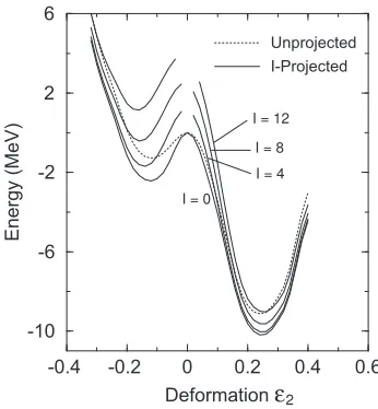
Nuclei are among the few quantum systems that can be discussed in terms of shape [1]. It is well-known that most nuclei in the nuclear chart are deformed. The most popu-lar type of deformation is axial-symmetric quadrupole de-formation. Calculations of total energies for such nuclei usually show a pronounced minimum at a certain defor-mation. Figure 1 illustrates a representative example from the 254No calculation, a well-deformed heavy nucleus in
the transfermium region. It is seen that deep minima are robustly developed at the deformation ε2 ≈ +0.25, no
matter if the calculation is performed with (solid curves) or without (dotted curve) angular momentum projection. Other local minima are well separated, lying by several MeV higher above the ground state. Therefore, this nu-cleus can be well regarded as a prolately-deformed rotor in the classical picture. In fact, a regular rotational band, with the band energies following the∼I(I+1) dependence expected from those of a classical rotor, has been observed experimentally [2].
Physics for such regularly-deformed nuclei can be de-scribed by models that choose the known deformation to construct a deformed basis. In their ground state, nuclei tend to couple their nucleons pairwise due to the pairing correlation. Thus, a deformed-quasiparticle (qp) basis ob-tained from the Nilsson+BCS calculation can be a good starting point to model such nuclear systems. Angular-momentum and particle-number projection can be incor-porated, respectively, to recover the violated rotational and gauge symmetries in the Nilsson and BCS calculations.
ae-mail: [email protected]
-0.4 -0.2 0 0.2 0.4 0.6 Deformation
ε
-10 -6 -2 2 6
Energy (MeV)
Unprojected I-Projected
2 I = 12
I = 8 I = 4 I = 0
Figure 1. Calculated angular-momentum-projected energy sur-faces for254No as functions of the quadrupole deformation pa-rameter. The unprojected calculation is given by the dotted curve.
Based on the deformed qp-vacuum, other configurations of qp excitations are included in the basis, and mixing of all these configurations is done by the shell model diago-nalization. This is the basic philosophy that the Projected Shell Model (PSM) follows [3].
Nuclear rotation tends to break the nucleon pairs due to the Coriolis antipairing effect [4]. The nucleon pairs in the orbitals with the highest angular momentum j, as for in-stance the neutroni13/2shell in the rare earth region, feel a
stronger Coriolis force, and therefore, break first [5]. They contribute to the formation of a 2-qp state as the main
con-C
Owned by the authors, published by EDP Sciences, 2015
-0.4 -0.2 0 0.2 0.4 0 2 4 6 8 10
Cd
I=0 I=2 I=4 I=6 I=8 I=10 110ε
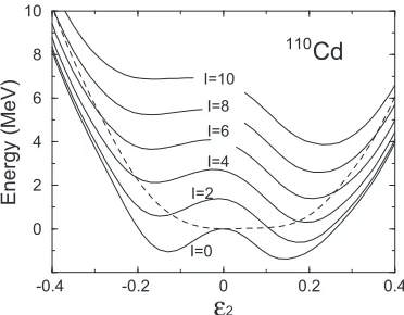
2 Energy (MeV)Figure 2. Calculated angular-momentum-projected energy sur-faces for110Cd as functions of the quadrupole deformation pa-rameter. The unprojected calculation is given by the dashed curve.
figuration of the yrast state. As a nucleus rotates faster and faster, subsequent pair-breakings can occur for the pairs from the next highest jorbitals. In the rare earth region, proton pairs in theh11/2 shell are expected to break next.
Further pair breakings at higher angular momenta are pos-sible, and there have been early [6] and recent evidences [7, 8] of breaking of three nucleon pairs, which form 6-qp states as the main configuration of the yrast sequence.
The difficulty to describe the above phenomena in a shell-model framework lies in the procedure of computing the overlap matrix elements [4] between arbitrary multi-qp states. Since the involved overlap matrix elements of multi-qp states are usually calculated with the generalized Wick’s theorem [3], one may encounter a problem of com-binatorial complexity when more than 4-qp states are in-cluded in the basis configurations. Therefore, to push the calculation further involving higher order of qp states, a breakthrough in computational many-body techniques is needed. In nuclear structure physics, the Pfaffian concept has been introduced [9] as a key mathematical tool for solving the long-standing problem in the phase determi-nation of the Onishi formula [10]. Moreover, it has been shown that the Pfaffian algorithm is very efficient also for calculating overlap matrix elements [11–16]. In particular, by means of Fermion coherent states and the Grassmann integral, one can derive an alternative approach to calcu-late the rotated matrix element for general qp states [17], which serves as a theoretical framework to extend the PSM model space [18].
However, there are many other nuclei either having multiple shapes coexisting near the ground state or being very soft without any simply-defined shapes [19]. Fig-ure 2 illustrates an example from the 110Cd calculation, a soft nucleus in the transitional region. It is seen that for this nucleus, the angular-momentum-projected and unpro-jected calculations show qualitatively different features. While the unprojected calculation (dashed curve in Fig. 2) suggests a spherical shape, the ground state obtained by the projected calculation shows competing prolate-oblate minima separated by only a small energy barrier.
More-over, as the nucleus rotates, the minima change towards larger absolute values; namely, the nucleus becomes more and more deformed [20]. Obviously for this kind of nu-clei, one can not build a shell model basis simply with one deformation. The correct way to describe such systems is to superimpose in the wavefunction all possible shapes described by different deformation parameters, which is a concept generally known in the literature as the Generater Coordinate Method (GCM) [4].
The present paper summaries the recent development of PSM based on the Pfaffian algorithm and the projected Generater Coordinate Method.
2 Application of the Pfaffian algorithm
2.1 The formalism
The PSM employs the Nilsson model [21] to generate a deformed single-particle basis. Pairing correlations are considered by a BCS calculation. The Nilsson-BCS cal-culation defines a deformed qp basis from which the PSM model space is constructed. The multi-qp configurations up to 6-qp states for even-even nuclei are given as [18]
|Φ,a†νia†νj|Φ,a†πia†πj|Φ, a†νia†νja†πka†πl|Φ, a†νia†νja†νka†νl|Φ, a†πia†πja†πka†πl|Φ,
a†νia†νja†νka†νla†νma†νn|Φ, a†πia†πja†πka†πla†πma†πn|Φ,
a†πia†πja†νka†νla†νma†νn|Φ, a†νia†νja†πka†πla†πma†πn|Φ. (1)
In the above expression,a†ν,a†π(aν,aπ) denote neutron and proton qp creation (annihilation) operators associated with the qp vacuum|Φ.
The PSM wave function is a linear combination of pro-jected states
|Ψσ I M=
Kκ
fIKσκPˆ I
MK|Φκ, (2)
where |Φκ are the qp-states in (1). ˆPI
MK is the angular momentum projection operator [4]
ˆ
PIMK = 2I+1
8π2
dΩDIMK(Ω) ˆR(Ω), (3)
with DIMK being theD-function, ˆR the rotation operator, andΩthe Euler angles. The energies and wave functions are obtained by solving the eigenvalue equation:
Kκ
HIKκ,Kκ−EσIN I Kκ,Kκ
fIKσ
κ =0, (4)
where HIKκ,Kκ andNKIκ,Kκ are the projected matrix ele-ments of the Hamiltonian and the norm respectively
HKIκ,Kκ=Φκ|HˆPˆIKK|Φκ, N I
Kκ,Kκ=Φκ|Pˆ I KK|Φκ.
(5)
The central task in numerical calculations is to evaluate rotated matrix elements of the Hamiltonian and the norm
with the operator [Ω]=Rˆ(Ω)/Φ|Rˆ(Ω)|Φ[3]. SinceHκκ
can be decomposed into terms expressed by the “linked" contraction andNκκ [3], the main task then concentrates on treating efficientlyNκκ. For the sake of convenience, we rewrite it as the following explicit form
Nκκ=Φ|a1· · ·an[Ω]a†1· · ·a†n|Φ, (7)
which is usually evaluated [3] by the generalized Wick’s theorem that decomposes Eq. (7) into a combination of three types of contractions, denoted asA,B, andC, with their matrix expressions [22]
Aνν(Ω)≡ Φ|[Ω]a†νa†ν|Φ,
Bνν(Ω)≡ Φ|aνaν[Ω]|Φ, (8)
Cνν(Ω)≡ Φ|aν[Ω]a†ν|Φ.
It was pointed out [17] that in applying the generalized Wick’s theorem, a matrix element of Eq. (7) involvingn
andnqps, respectively in the left- and right-side of [Ω],
contains (n+n−1)!! terms. In practice, the number of terms becomes so large that it is nearly impossible to write down expressions explicitly for more than 4-qp states.
By using the Fermion coherent state and the Grass-mann integral, a general expression for the matrix ele-ments (7) in terms of the Pfaffian can be derived [17]
Φ|a1· · ·an[Ω]a†1· · ·a†n|Φ=P f(X)=P f
B C
−CT A , (9)
whereXis a skew-symmetric matrix with dimension (n+ n)×(n+n). The indices of rows and columns forBrun from 1 ton (1, . . . ,n) and the ones forArun from 1 to
n(1, . . . ,n). For the matrixCin Eq. (9), the indices of rows run from 1 tonand those of columns run from 1to
n. The Pfaffian is defined as
P f(A)≡ 1
2nn!
σ∈S2n
sgn(σ) n
i=1
aσ(2i−1)σ(2i). (10)
for a skew-symmetric matrixAwith dimension 2n×2n, of which matrix elements areai j. The symbolσis a per-mutation of {1,2,3, . . .,2n}, sgn(σ) is its sign, and S2n represents a symmetry group. This makes it possible and efficient to work with the expanded PSM configuration in (1), since calculations of the corresponding Pfaffian are not time-consuming [23].
2.2 The166Hf example
The PSM employs the Hamiltonian with separable forces:
ˆ
H=Hˆ0−
1 2χQQ
μ ˆ
Q†2μQˆ2μ−GMPˆ†Pˆ−GQ
μ ˆ
P†2μPˆ2μ,
(11)
where ˆH0 is the spherical single-particle term
includ-ing the spin-orbit force [24], and the rest is the quadrupole+pairing type of interactions, which contains
Figure 3. (Color online) Back-bending plot for166Hf. The cal-culated results are compared with the data taken from Ref. [7]. This figure is taken from Fig. 1 of Ref. [18].
three parts. The strength of the quadrupole-quadrupole term χQQ is related to deformation of the basis [3]. The monopole-pairing strength is taken to be the formGM = [G1 ∓G2(N −Z)/A]/A, where “+" (“−") is for protons
(neutrons), withG1 = 20.12 andG2 = 13.13 being the
coupling constants [3], in correspondence to the full con-figuration space of three major harmonic-oscillator shells,
N = 4,5,6 (N = 3,4,5) for neutrons (protons). The quadrupole-pairing strength GQ is taken, as usual, to be 16% ofGMfor all the nuclei considered in this study.
The anomalies in the observed moment of inertia (MOI) of a rotating nucleus are usually displayed in an exaggerated manner with a back-bending plot, in which twice the MOI, 2Θ, is plotted as a function of the square of the rotational frequencyω2. Figure 3 shows the back-bending plot for 166Hf, where the theoretical results are compared with the experimental data. In the calculation, the deformation parameters are fixed asε2 = 0.208 and
ε4 = 0.013 which are taken from Ref. [25].
Anoma-lies in MOI can be clearly seen asωincreases, roughly at ω2≈0.10, 0.15 and 0.25, corresponding to spinI≈12, 24
and 34, respectively. The first anomaly exhibits the largest effect, causing a sharp increase in 2Θ. This is known as the first back-bending, corresponding to breaking and align-ment of a neutroni13/2pair. The second anomaly in Fig.
3 corresponds to the small increase in 2Θatω2 ≈ 0.15,
which is nicely reproduced by the calculation. At this ro-tational frequency, an additionalh11/2 proton pair is
bro-ken and their spins are aligned along the axis of rota-tion. The third anomaly belongs to the few known cases that have ever been observed: 2Θjumps suddenly again atω2 ≈ 0.25. The observation is correctly described by the present calculation, and is understood as the additional breaking of a second neutroni13/2pair. Therefore above
this point the yrast line consists of a 6-qp configuration with two qp-pairs in the neutroni13/2shell and one qp-pair
in the protonh11/2shell.
Figure 4. (Color online) Band diagram for 166Hf. Note that only even-spin states are plotted in order to avoid zigzag in these curves. This figure is taken from Fig. 2 of Ref. [18].
as
Eκ(I)=Φκ| ˆ
HPˆI KK|Φκ Φκ|PˆI
KK|Φκ
, (12)
which is the projected energy of a multi-qp configuration in (1). Figure 4 displays the band diagram for166Hf, where the 0-qp ground (g-) band, one 2-qp band, one 4-qp band, and three 6-qp bands are selected from about 200 projected configurations because of their important roles played in the yrast band (marked by dots). It is seen that the first back-bending atI≈12 in Fig. 3 corresponds to the cross-ing between g-band and the 2-qp (s-) band. The configura-tion of thes-band is found to beν3/2+[651]⊗ν5/2+[642] with K = 1. The s-band remains to be the yrast band until it is crossed by a 4-qp band at I ≈ 24. This 4-qp band is based on an addition of an h11/2 proton pair,
corresponding to the configurationν3/2+[651]5/2+[642]⊗ π7/2−[523]9/2−[514] withK =2. The third anomaly in MOI corresponds to the crossing of the 4-qp band with three 6-qp bands atI≈34. Two of the 6-qp bands whose energies are almost the same at low spins have the same configurationν1/2+[660]3/2+[651]5/2+[642]7/2+[633]⊗ π7/2−[523]9/2−[514] but with different K values K =
−1 and −3. The configuration of the third 6-qp band is ν1/2+[660]3/2+[651]5/2+[642]5/2+[642] ⊗ π7/2−[523]9/2−[514] with K = 0. As the level density increases with spin, the wave function of the yrast band beyondI≈34 is found to have a large admixture of these 6-qp states.
3 Generater Coordinate Method
While the above discussed method is powerful for nuclei with a well-defined stable shape, it can not be applied to transitional nuclei which either have multiple shapes coex-isting near the ground state or are so soft that one can not even talk above shapes. Quite recently, we have improved
Figure 5. (Color online) Comparison of the calculated 0+2 state with experimental data for Gd, Dy, and Er isotopes. The energy levels 2+1, 4+1, and 6+1 of the ground-state rotational band are also shown. Calculated results (open circles) are compared with data (filled squares). This figure is taken from Fig. 1 of Ref. [26].
the PSM wavefunction by using the Generater Coordinate Method (GCM) [26].
3.1 GCM Theory
To improve the wavefunction (2) which corresponds to a fixed quadrupole deformationε2, a better wave function
can be constructed by takingε2as the generate coordinate
|ΨI,N=
dε2fI,N(ε2) ˆPIPˆN|Φ(ε2), (13)
where ˆPNis the particle-number projection operators. The weight fI,N(ε2) is determined by the diagolnalization.
3.2 GCM examples
In Fig. 5, we show the results of a systematic calculation for the first excited 0+2state in Gd, Dy, and Er isotopes, and compare them with experimental data. The energy levels 2+1, 4+1, and 6+1 of the ground state rotational band are also shown. We find that with a single set of parameters in the Hamiltonian, the characteristic behavior of the shell evo-lution is well reproduced. This certainly benefits from the improved GCM wave function of Eq. (13). It is seen that starting from the neutron numberN =90 on the l.h.s. of Fig. 5 and going to heavier isotopes the ground state bands becomes more and more compressed, eventually following the rotational rule ofE∼I(I+1) atN=98. On the other hand, the 0+2 state is found low for the isotopes with neu-tron number 90, which are thought to be soft nuclei with low-energy vibrational states. Without any adjustable pa-rameter, the increase of the energy of the 0+2 state with increasing neutron number is correctly reproduced for all three isotopic chains, thus clearly distinguishing the spec-tral differences of softness in lighter isotopes and stiffness in heavier isotopes, with regard to deformation. The case with the largest discrepancy between calculation and data is158Er, which is known to be relatively soft in triaxiality.
We may conclude that the improved GCM wave function of Eq. (13) is able to describe correctly both soft and stiff nuclei, and the transition between them.
4 Summary
This paper summarizes the recent developments of PSM by using the many-body techniques, which allow to de-scribe rotationally induced structural changes at very high spins and shape evolutions between the soft to well-deformed nuclei. On one hand, the configuration space of PSM has been expanded considerably by using the Pfaffian algorithm. On the other hand, the angular-momentum-projected GCM has been developed based on the PSM framework, which largely enriched the PSM wavefunc-tions. A combination of these two developments, namely the construction of multi-qp configurations on top of the GCM states, is under our consideration.
Acknowledgements
Research at SJTU was supported by the National Natural Science Foundation of China (No. 11135005) and by the 973 Program of China (No. 2013CB834401).
References
[1] A. Bohr and B. R. Mottelson,Nuclear Structure, Vol. 2 (Benjamin, New York, 1975)
[2] R.-D. Herzberg and P. T. Greenlees, Prog. Part. Nucl. Phys.61, 674 (2008)
[3] K. Hara and Y. Sun, Int. J. Mod. Phys. E4, 637 (1995) [4] P. Ring and P. Schuck,The nuclear many-body
prob-lem(Springer Verlag, Berlin, 2004)
[5] F. S. Stephens and R. S. Simon, Nucl. Phys. A 183, 257 (1972)
[6] J. Burdeet al., Phys. Rev. Lett.48, 530 (1982) [7] D. R. Jensenet al., Eur. Phys. J. A8, 165 (2000) [8] R. B. Yadavet al., Phys. Rev. C80, 064306 (2009) [9] L. M. Robledo, Phys. Rev. C79, 021302(R) (2009) [10] N. Onishi and S. Yoshida, Nucl. Phys.80, 367 (1966) [11] L. M. Robledo, Phys. Rev. C84, 014307 (2011) [12] G. F. Bertsch and L. M. Robledo, Phys. Rev. Lett.
108, 042505 (2012)
[13] B. Avez and M. Bender, Phys. Rev. C 85, 034325 (2012)
[14] M. Oi and T. Mizusaki, Phys. Lett. B707, 305 (2012) [15] T. Mizusaki and M. Oi, Phys. Lett. B715, 219 (2012) [16] Q.-L. Hu, Z.-C. Gao, and Y. S. Chen, Phys. Lett. B
734, 162 (2014)
[17] T. Mizusaki, M. Oi, F. Q. Chen, and Y. Sun, Phys. Lett. B725, 175 (2013)
[18] L.-J. Wang, F.-Q. Chen, T. Mizusaki, M. Oi, and Y. Sun, Phys. Rev. C90, 011303(R) (2014)
[19] K. Heyde and J. L. Wood, Rev. Mod. Phys.83, 1467 (2011)
[20] P. H. Reganet al., Phys. Rev. Lett.90, 152502 (2003) [21] S. G. Nilssonet al., Nucl. Phys. A131, 1 (1969). [22] K. Hara and S. Iwasaki, Nucl. Phys. A 332, 61
(1979).
[23] C. González-Ballestero, L. M. Robledo, and G. F. Bertsch, Comput. Phys. Commun.182, 2213 (2011) [24] T. Bengtsson and I. Ragnarsson, Nucl. Phys. A436,
14 (1985)
[25] P. Moller, J. R. Nix, W. D. Myers, and W. J. Swiate-cki, At. Data Nucl. Data Tables59, 185 (1995) [26] F.-Q. Chen, Y. Sun, and P. Ring, Phys. Rev. C 88,
014315 (2013)
[27] T. R. Rodríguez and J. L. Egido, Phys. Lett. B705, 255 (2011)
[28] J. M. Yao, M. Bender, and P.-H. Heenen, Phys. Rev. C87, 034322 (2013)
[29] Y. Fuet al., Phys. Rev. C87, 054305 (2013)
[30] J.-P. Delaroche et al., Phys. Rev. C 81, 014303 (2010)