o f
F
i n a n c i a lM
a r k e tR
i s k a n dL
i q u i d i t yA thesis submitted to the Department of Finance of the
London School of Economics and Political Science
for the degree of PhD in Finance
London School of Economics and Political Science,
September 2008
All rights reserved
INFORMATION TO ALL USERS
The quality of this reproduction is dependent upon the quality of the copy submitted.
In the unlikely event that the author did not send a complete manuscript and there are missing pages, these will be noted. Also, if material had to be removed,
a note will indicate the deletion.
Dissertation Publishing
UMI U615677
Published by ProQuest LLC 2014. Copyright in the Dissertation held by the Author. Microform Edition © ProQuest LLC.
All rights reserved. This work is protected against unauthorized copying under Title 17, United States Code.
ProQuest LLC
789 East Eisenhower Parkway P.O. Box 1346
I certify th a t the thesis I have presented for examination for the
PhD degree of the London School of Economics and Political Science
is solely my own work other than where I have clearly indicated that
it is the work of others (in which case the extent of any work carried
out jointly by me and any other person is clearly identified in it).
The copyright of this thesis rests with the author. Quotation from
it is permitted, provided th at full acknowledgement is made. This
thesis may not be reproduced without the prior written consent of the
author.
I warrant th at this authorisation does not, to the best of my belief,
infringe the rights of any third party.
my mother, my father, my sisters, my grandparents, for always believing in me and helping me be who I am.
This thesis provides a novel empirical treatm ent of the dynamics of
financial market risk and liquidity, two very im portant areas both for
financial research as well as to practitioners in the financial markets:
We devise empirical non-linear time series models of the two concepts
th at specifically take into account ‘explosive’, self-reinforcing dynamic
patterns. While ‘conventional’ empirical models are often ‘linear’ and
tend to neglect these effects, real-life evidence such as e.g. the 1987
crash, the large stock market drops on February 27th, 2007 or the huge losses posted by investment banks and hedge funds during July and
August 2007, suggest th at such an approach is warranted:
In the first part of the thesis we extend a time series model of
Value-at-Risk (VaR) with non-linear multiplicative features and en
dogenous regime thresholds. When estimated with a Markov Chain
Monte Carlo (MCMC) method against real data, the resulting ‘Self-
Exciting Threshold CAViaR’ (Conditional Autoregressive Value-at-
Risk) model is able to detect trigger thresholds for explosive market
risk as well as the scale of such a possible expansion in risk.
The second part of the thesis is dedicated to the ‘Conditional Au
toregressive Liquidity’ (CARL) model, a multiplicative time series ap
proach to the empirical modelling of market liquidity. The newly con
ceptualised model is capable of picking up self-reinforcing dynamics,
i.e. autoregressive patterns in liquidity, which is in accordance with
theoretical research on the topic. Moreover, by incorporating a multi
dimensional liquidity proxy, the model CARL is explicitly designed to
take into account the fact th at liquidity is a concept with many facets,
unlike other empirical treatm ents th a t often view liquidity only along
a single dimension (e.g. the bid-ask spread, volume, trade duration).
In this thesis, we demonstrate the empirical versatility of the model
using both fixed interval data (daily and weekly) as well as tick-by-tick
intraday data, for which we propose a filtering technique in order to be
able to use the model in such a data environment. We note th at the
model is able to pick up autocorrelation structures in liquidity rather
well and find the forecast performance very encouraging for practical
This doctoral thesis would not be without the help and support of
many. You know who you are! It shames me to admit th a t I will cer
tainly forget to mention quite a few of you explicitly below. However,
do rest assured th a t I am very much indebted to all of you and will
always be grateful for your help and advice. In this limited space, I
will merely try to highlight those th at I owe most.
First and foremost, I would like to express my deepest gratitude
to Dr. Jon Danielsson, my academic supervisor and mentor for many
years. These few words cannot possibly capture how much I am in
debted to him for his support. I met Jon already while being an
undergraduate at the LSE and he has been a invaluable source of help
and advice ever since. Many skills as a researcher, especially in scien
tific programming, I have learned from him. They will stay with me
for the years to come.
I also wish to thank my second supervisor Dr. Andrew Patton, Prof.
Greg Connor, Prof. Oliver Linton as well as Dr. Antonio Mele for their
advice and help in showing me new avenues of progress and keeping
me going when things got difficult. In this respect, I would also like to
express my gratitude to the participants in the PhD Finance seminar
and the Wednesday Econometrics workshop, especially Dr. Michaela
Verardo, Dr. Christian Julliard and Prof. Antoine Faure-Grimaud,
for their helpful comments, advice and encouragement.
I also owe a special mention to Prof. David Webb to whom I am
particularly grateful. I have known David since being an undergradu
ate at the LSE. His help, advice and understanding - also in areas other
than academia - have kept me going, helped me become a successful
researcher and make the most of my time at the Financial Markets
Group.
My gratitude also extends to Dr. Sushil Wadhwani for his interest
in my work and providing with an excellent professional perspective
for the time after my research studies.
I would like to thank the London School of Economics and the
Financial Markets Group, especially Mary Comben, Maria Komninou,
Sooraya Mohabeer and Osmana Raie for providing me with excellent
resources for my research and helping me find my way through LSE’s
administrative ‘jungle’. The generous financial support by Concordia
Advisors during the third year of my PhD studies is also gratefully
acknowledged.
I have always been able to rely on my family, my mother, my father,
my sisters and my grandparents for support. They have never stopped
to encourage me and lifted me up when I was at loose ends. They are
the people who have allowed me to pursue my dreams and become
who I am today. To them I am indebted beyond words. It pains me
especially that my grandparents are not with me anymore to witness
what they have greatly supported me in doing. It is to them th at I
unconditional love and support.
I would also like to express my gratitude to Jana Klimecki who has
been a tremendous source of inspiration and motivation during some
of the difficult phases of my work. She kept me going in my efforts to
produce research of the highest quality.
Erwin Bechtold used to be my English teacher at the Tilemannschule
in Limburg. It is largely also because of him th at I was able to start
my studies at the LSE in the first place. I owe him many thanks for
that.
Finally, I would like to thank Mohammed Fawaz, Anisha Gosh, Dr.
Georg Kaltenbrunner, Dr. Manuel Klein, Ossi Lindstrom, Dr. Ryan
Love, Ebrahim Rahbari, Dr. Miguel Segoviano and Bernhard Silli for
being good friends and helpful colleagues. Anisha has often helped me
grasp the odd difficult notion in (asymptotic) econometrics. My con
versations with Georg, Manuel, Ossi, Ebrahim, Miguel and Bernhard
have greatly shaped my understanding of financial economics, the aca
demic world and the financial industry. And, without Mohammed and
1 In trod u ction 16
2 S elf-E xciting CAV iaR M od els w ith E ndogenous T hresh
olds 23
2.1 In tro d u c tio n ... 23
2.2 CAViaR and Quantile (A uto-)R egression... 29
2.2.1 Quantile Estimation ... 29
2.2.2 The General CAViaR M o d e l... 30
2.2.3 Popular CAViaR M o d e ls ... 30
2.3 CAViaR in Relation to ARMA-GARCH ... 32
2.4 The Self-exciting Threshold CAViaR Model ... 35
2.4.1 Endogenous Self-Reinforcing R i s k ... 36
2.4.2 The Case for Self-exciting Non-linear Dynamics 37 2.4.3 S E T -C A V iaR ... 40
2.5 MCMC L T E ... 46
2.5.1 MCMC LTE D e t a i l s ... 49
2.5.2 Cooling the ‘Temperature’ ... 52
2.5.3 Monitoring Chain P e rfo r m a n c e ... 54
2.5.4 Statistical Inference... 57
2.6 A Monte Carlo S tu d y ... 59
2.7 Empirical Application ... 67
2.7.1 Data D e s c rip tio n ... 67
2.7.2 Implementation and C o m p u tin g ... 70
2.7.3 Model S e tu p ... 73
2.7.4 Estimation Results for 95% VaR (r = 0.05) . . 74
2.7.5 Estimation Results for 99% VaR (r = 0.01) . . 85
2.7.6 Discussion of R e s u lts ... 96
2.8 Conclusion...102
3 CARL: A n E m pirical C onditional A u toregressive M odel o f M arket L iquidity 111 3.1 In tro d u c tio n ... I l l 3.2 Liquidity in Financial M a rk e ts...115
3.2.1 The Theory C o n t e x t ...119
3.2.2 The Empirical C o n te x t...124
3.3 Two Building B lo c k s ...130
3.3.1 A Multi-Dimensional Liquidity Measure . . . . 130
3.3.2 The Econom etrics... 136
3.4 The CARL M o d el... 137
3.4.1 Model S e tu p ...137
3.4.2 Asymptotic Properties and E s tim a tio n ... 140
3.4.3 Theoretical Underpinnings and Extensions . . . 143
3.5 Empirical Application ...146
3.5.1 D a t a ... 146
3.5.2 Estimation and R e su lts... 151
3.5.3 D iscussion... 164
3.6 Conclusion...169
4.2 Intraday Market L iq u id ity ... 183
4.2.1 Econometric Model B ackground... 185
4.3 Intraday Liquidity a la C A R L ...189
4.3.1 The HH Ratio R e v is ite d ...190
4.3.2 The Maximum Percentage Range Measure . . . 191
4.3.3 The CARL Model R e v is ite d ...196
4.4 D a t a ... 197
4.4.1 F ilte r in g ... 202
4.4.2 Market Microstructure I s s u e s ... 209
4.5 Empirical Application ...212
4.5.1 Intermediate Volume (m = 500) ... 213
4.5.2 Varying the Transaction Filter S i z e ...216
4.5.3 D iscussion... 228
2.1 T G A R C H (1,1) param eter e s t i m a t e s ... 61
2.2 P aram eter linkages SE T -C A V iaR ... 63
2.3 E r r S c o re^2 for different sca le/th resh o ld com bi
n ations ... 65
2.4 C R S P IB M holding return d ata sta tistic s . . . . 70
2.5 SE T -C A V iaR param eter estim ates ( r = 0.05) . . 75
2.6 SE T -C A V iaR param eter estim ates (r = 0.01) . . 86
3.1 A m azon H H ratio, return and turnover data
s t a t i s t i c s ... 148
3.2 E stim ation - 1997-2006 daily A m azon d ata . . . 153
3.3 E stim ation - 2001-2006 daily A m azon d ata . . . 154
3.4 MZ - 1997-2006 daily A m azon d a t a ...160
3.5 MZ - 2001-2006 daily A m azon d a t a ...160
3.6 E stim ation - 1997-2006 w eekly A m azon d ata . . 162
3.7 MZ - 1997-2006 w eekly A m azon d a t a ... 165
4.1 Intraday A m azon data sta tistics (2 4 /0 7 /2 0 0 1 ) . 200
4.2 S ta tistics - F iltered intraday A m azon rm t series
(m = 500) 205
4.3 E stim ation - F iltered intraday A m azon rmjt se
ries (m = 5 0 0 ) ... 214
4.4 MZ - F iltered A m azon rm>t series (m = 500) . . . 216
4.5 C om parative sta tistics - F iltered A m azon rm t se
ries ...217
4.6 E stim ation - D ifferent filtered intraday A m azon
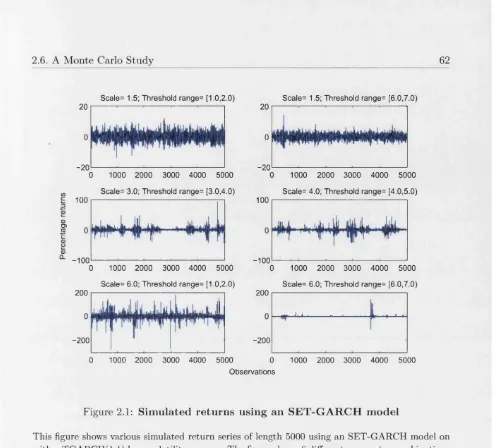
2.1 Sim ulated returns using an SE T -G A R C H m od el 62
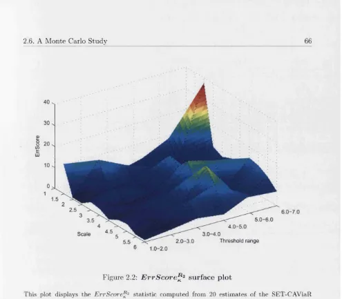
2.2 E r r S c o r e ^ 2 surface p l o t ... 66 2.3 C R S P IB M holding r e t u r n s ... 69
2.4 C R S P IB M holding returns h i s t o g r a m ... 71
2.5 A verage au tocorrelation functions ( r = 0.05) . . 80 2.6 SE T -A S-C A V iaR para’s (r = 0 . 0 5 ) ... 81
2.7 SE T -G JR -IG A R C H -C A V iaR para’s ( r = 0.05) . 82
2.8 SE T -A S-C A V iaR posteriors (r = 0.05) 83
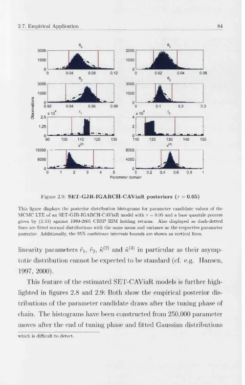
2.9 S E T -G JR -IG A R C H -C A V iaR p osteriors (r = 0.05) 84
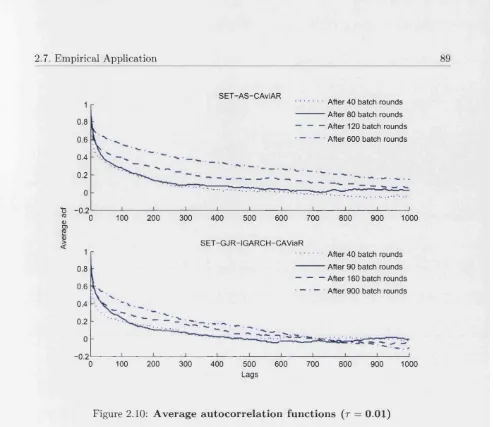
2.10 A verage au tocorrelation functions (r = 0.01) . . 89
2.11 SE T -C A V iaR likelihood evolu tion ( r = 0.01) . . . 90
2.12 SE T -C A V iaR likelihood ev olu tion ( r = 0.05) . . . 91
2.13 SE T -A S-C A V iaR para’s ( r = 0 . 0 1 )... 92
2.14 SE T -G JR -IG A R C H -C A V iaR para’s ( r - 0.01) . 93
2.15 SE T -A S-C A V iaR posteriors (r = 0.01) 94
2.16 SE T -G JR -IG A R C H -C A V iaR posteriors ( r = 0.01) 95
3.1 M arket liquidity - T ightness and d e p t h ...133
3.2 A m azon H H ratio, return and tu r n o v e r ...149
3.3 H istogram and A C F - 1997-2006 daily A m azon
H H r a t i o ...152
3.4 H istogram and A C F - 2001-2006 daily A m azon
H H r a t i o ... 155
3.5 A ctu al vs Forecast - 1997-2006 daily A m azon
H H r a t i o ...158
3.6 A ctu al vs Forecast - 2001-2006 daily A m azon
H H r a t i o ...159
3.7 H istogram and A C F - 1997-2006 w eekly A m azon
H H r a t i o ...161
3.8 A ctu al vs Forecast - 1997-2006 w eekly A m azon
H H r a t i o ...163
4.1 A m azon daily price, p ercentage range, return
and v o l u m e ... 199
4.2 A m azon adj transaction price, volum e and
bid-ask s p r e a d ...201
4.3 A m azon intraday b u y /se ll price and volum e . . . 204
4.4 H istogram & A C F - A m azon rm t (m = 500) . . . 207
4.5 A m azon rm t and O IB m?* (m = 5 0 0 ) ... 208
4.6 H istogram & A C F - A m azon rm t (m = 100) . . . 218
4.7 A m azon rm t and 0 1 B m t (m = 1 0 0 ) ...219 4.8 H istogram &: A C F - A m azon rm t (m = 1,00 0) . . 220
4.9 A m azon rm?t and O IB m^ (m = 1,000) 221
4.10 H istogram &: A C F - A m azon rm?t (m = 1 0,000) . 222
In trod u ction
This thesis provides a novel empirical treatm ent of the dynamics of
financial market risk and liquidity, two very im portant areas both for
financial research as well as to practitioners in the financial markets:
We devise empirical non-linear time series models of the two concepts
th at specifically take into account ‘explosive’, self-reinforcing dynamic
patterns. While ‘conventional’ empirical models are often ‘linear’ and
tend to neglect these effects, adverse events in the history of the fi
nancial markets suggest th at such an approach is warranted:
On February 27^, 2007 for example, the Dow Jones Stoxx 600
Index dropped by 3% in a manner that, according to the The Wall Street Journal Europe, edn. February 28th, 2007, was “almost like (...) a cascade” . Regarding these events, The Economist, issue March 3 rd, 2007, pointed out th at investment banks often sell assets when volatility is rising in a move to cut capital allocated to trading, thereby
creating self-reinforcing patterns in market risk: ” ...a sudden jump
in volatility tends to generate further volatility” , resulting in a large
build-up of risk and potentially large losses. Another example for
these mechanisms at work are the events in July and August 2007,
when many investment banks and hedge funds posted major losses on
their trading books: Goldman Sachs’ main equity fund for example
lost more than 30% of its value in a week caused by problems in its
computer-driven trading strategies. The Financial Times on August 14th 2007, analyses:
“The issue of computer ‘herding’ appears to be a key factor
behind this m onth’s [August 2007] problems at the Goldman
Sachs funds and others (...) computer models do not always
take account of the way th at their own behaviour is affecting
markets (...) In practical terms, this means th at when mod
els evaluate markets, they often fail to recognise how their
own behaviour is distorting prices (...) Computers have a
nasty habit of all using similar strategies - partly because
they are created by humans who have studied at the same
institutions. Thus they can all dash for the exits at the same
time.”
Regarding the losses th at materialised as a result of these issues,
Goldman Sachs’ chief financial officer, Mr. Davir Vaniar comments in
the same paper:
“We are seeing things th at were 25-standard deviation events,
several days in a row.”
W ith a more explicit focus on liquidity, The Economist, edn. April 28th, 2007 states:
“Liquidity is a self-reinforcing process (...) if liquidity sud
denly dries up, some investors might end up owning assets
they neither want nor can get rid of. This might make a
Carlson (2007) further suggests th at such liquidity problems were
also hat the heart of the 1987 market crash. He argues th a t so-called
margin calls on trading positions th at suffered from losses, led to re
duced market liquidity in the (futures) market through further selling,
which in turn led to an even steeper decline.
The above evidence from the financial markets thus suggests th at
market risk and (il)liquidity are subject to feedback ‘loops’ as well as
‘cross-over’ effects, whereby market risk and (il)liquidity may feed on
themselves and each other to create explosive patterns th a t can ad
verse affect trading conditions. This mechanism has been documented
by Danfelsson and Shin (2003) and themed ‘endogenous risk’. Morris
and Shin (1998), Morris and Shin (2004) as well as Brunnermeier and
Pedersen (2008) have provided theoretical models of these feedback
mechanisms th at can lead to liquidity ‘black holes’, excessive market
risk and potentially large price drops in asset markets.
In this thesis we seek to develop new empirical time series models of
market risk and liquidity th at capture these ‘unorthodox’ dynamics:
In the first part of the thesis we extend a time series model of Value-at-
Risk (VaR) with non-linear multiplicative features and regime thresh
olds, to yield a non-linear time series model th a t is capable of estimat
ing explosive patterns in market risk.
The second part of the thesis is dedicated to the ‘Conditional Au
toregressive Liquidity’ (CARL) model, a multiplicative time series ap
proach to the empirical modelling of market liquidity. The newly
conceptualised model is capable of picking up self-reinforcing dynam
ics, i.e. autoregressive patterns in liquidity, in daily, weekly as well as
intraday data. Moreover, in the setup of our model we explicitly take
th a t are of varying importance both to different market participants
and over time: Thus, as a liquidity proxy in the CARL model, we use
the Hiu-Heubel liquidity ratio, a multi-dimensional measure of liquid
ity th at proxies for the tightness as well as depth and breadth of a
market.
Chapter 2 - Self-Exciting CAViaR M odels w ith Endogenous Thresholds
This chapter introduces the empirical model class of ‘Self-exciting
Threshold’ CAViaR (SET-CAViaR), in which threshold variables are
determined endogenously. The proposed model is designed to incor
porate reinforcing, explosive dynamics of market risk th at are referred
to as ‘endogenous risk’ and have recently received increased attention
in the theoretical literature as well as among practitioners. As such,
the SET-CAViaR constitutes a new empirical approach to risk mod
elling, which due to its semi-parametric and non-linear features calls
for a Markov Chain Monte Carlo (MCMC) estimation routine. We il
lustrate the model in a Monte Carlo study and estimate it with CRSP
IBM holding returns from 1982-2005. The estimation results generally
indicate a good fit and are well in accordance with theoretical predic
tions: There is evidence for the SET-CAViaR model detecting sudden,
explosive patterns in market risk, which ‘conventional’ models are not
conceived to pick up.
Chapter 3 - CARL: An Empirical Conditional A utoregressive M odel of Market Liquidity
In this chapter we present the Conditional Autoregressive Liquidity
(CARL) model, an empirical time series model of market liquidity. We
economet-ric framework, we use the multiplicative setup of Engle and Russell’s
(1998) ACD model; as a proxy for liquidity, we rely on the Hui-Heubel
ratio, a multi-dimensional measure of (il)liquidity th at captures many
facets of market liquidity. For the resulting CARL model, we estab
lish the econometric properties and demonstrate its empirical validity
in the light of recent theoretical research in financial liquidity: Such
theory predicts (il)liquidity to be self-reinforcing, thus strongly auto
correlated through time. In an empirical application using both daily
as well as weekly CRSP Amazon data from 1997-2006 we find th at the
CARL model picks up such autocorrelation rather well and produces
accurate forecasts.
Chapter 4 - Intraday Liquidity: A High-Frequency A pplication o f th e CARL M odel
This chapter constitutes an application of the CARL model to an in
traday context. In order to use the model in a high-frequency data
environment characterised by irregular time intervals between subse
quent tick-by-tick observations, we propose a volume technique: We
sort data into volume durations during which a particular volume is
both bought and sold and derive the maximum percentage range liq
uidity measure, a metric similar to the Hui-Heubel ratio, over the
resulting intervals. The filtered series is then taken as an input into
the CARL framework. We demonstrate the filtering technique as well
as the versatility of the resulting intraday CARL model in an empirical
application using TAQ intraday data on Amazon: Similar to previous
empirical work in a daily and weekly data context and in line with
theoretical research, we find th at the model is able to pick up signif
Brunnermeier, M. and Pedersen, L. H. (2008), Market liquidity and
funding liquidity. Working paper, Princeton University; forth
coming in the Review of Financial Studies; available from h t t p : / / www.p r in c e to n .e d u /~ m a r k u s /r e s e a r c h /p a p e r s /liq u id ity .
Carlson, M. (2007), A brief history of the 1987 stock market crash:
with a dicussion of the Federal Reserve response, The finance
and economics discussion series (feds) papers, The Federal Re
serve Board; available from h ttp ://w w w .fe d e r a lre s e r v e .g o v /
pubs/feds/2007/200713/200713pap. pdf.
Danfelsson, J. and Shin, H. S. (2003), Endogenous risk, in P. Field, ed., ‘Modern Risk Management’, Risk Books, London, UK, pp. 297-316.
Engle, R. F. and Russell, J. R. (1998), ‘Autoregressive conditional du
ration; a new model for irregularly spaced transaction d a ta ’, Econo-metrica 66, 1127-1162.
Morris, S. and Shin, H. S. (1998), ‘Unique equilibrium in a model of
self-fulfilling currency attacks’, American Economic Review 88, 587- 597.
Morris, S. and Shin, H. S. (2004), ‘Liquidity black holes’, Review of Finance 8, 1-18.
S elf-E xcitin g C A V iaR M od els w ith
E ndogenous T hresholds
2.1
Introduction
Most commonly used empirical models of market risk focus on the
quantification of such risk in terms of ‘Value-at-Risk’ (VaR), i.e. the
quantile of the returns distribution, through non-parametric empirical
estimation or using time series models in linear single-regime setups.
An example of an approach of the former kind is the popular method
of ‘Historical Simulation’ (HS), whereas the latter includes quantile
models based on conditional volatility or the ‘Conditional Autore
gressive Value-at-Risk’ (CAViaR) model class. Recently developed by
Engle and Manganelli (2004), CAViaR constitutes a semi-parametric
autoregressive quantile regression approach, whereby the conditional
quantile of the returns distribution at time t is typically directly mod elled as a function of lagged values of the return and its lagged own
conditional quantiles.
However, despite the wide-spread use, appeal and individual merits
(in the case of CAViaR, cf. Engle and Manganelli, 2004), the above
models are ill-equipped to incorporate self-exciting, reinforcing pat
terns in market risk, which recent theoretical research has dubbed
‘endogenous risk’: Damelsson and Shin (2003) for example suggest
th a t traders’ selling decisions can lead to self-exciting downward spi
rals in asset prices, thus creating endogenous risk from within the
financial system. More formally, Morris and Shin (1999) and Morris
and Shin (2004) show how coordination effects and higher order be
liefs along the lines of Morris and Shin (1998) can create endogenous
risk and ‘liquidity blackholes’: Once certain thresholds are crossed the
reinforcing actions of market participants can trigger to self-exciting
patterns and endogenous downward spirals in asset returns.
Building on the CAViaR model class, in this chapter we provide
a new framework in which to analyse endogenous risk empirically:
We propose the ‘Self-exciting Threshold’ CAViaR (henceforth SET-
CAViaR) model, an empirical time series model th at explicitly allows
for explosive, self-exciting risk dynamics over a part of the returns do
main. When estimated with real data, the new model is able to detect
‘trigger’ thresholds for self-exciting endogenous risk and is therefore
capable of identifying and predicting potential endogenously created
crises. Further, the model also quantifies the scale of endogenous risk
during such states of the world.
While the theoretical findings underlying the proposed SET-CAViaR
model have been known for some time, an empirical attem pt at provid
ing a framework for the analysis of endogenous risk as in this chapter
has to our knowledge so far not been attem pted. Yet, the practical
experience in financial markets also suggests th at such an approach is
82 th at on this day “[the Dow Jones Industrial Average] plummeted
[at] a rate of decline th at traders said was unprecedented” , suggesting
mutually reinforcing sell decisions by traders leading to a cascading
sell-off. The paper further concludes th at “if conventional [VaR] mod
els are correct, such an event should not have happened in the history
of the known universe” , indicating the need for better VaR modelling
methodologies in the face of such events.
We would argue th at the introduction of the SET-CAViaR model
represents a first step into this direction: The proposed methodology
builds on the CAViaR model as a univariate quantile ‘baseline’ process,
which we combine with a multiplicative scaling factor th a t is allowed
to differ across regimes. Regime shifts are triggered by lagged returns
crossing endogenously estimated thresholds. In this setup, risk - as
measured by the return quantile - can therefore increase exponentially
once an explosive regime is entered.
By relying on the recently developed CAViaR model, we benefit
from its semi-parametric properties: Specifying the law of motion of
the return distribution quantiles directly, CAViaR models the evolve-
ment of all moments of return distribution at different quantile levels - without the (ad hoc) assumption of a particular error term distribu
tion. In this respect, CAViaR contrasts with more ‘traditional’ empir
ical risk modelling methods based on models for conditional volatil
ity: Particular examples of the latter include models in the ARMA-
GARCH class1, which explicitly lay out the law of motion of the first
and second moments of the returns distribution, but do not address higher moment dynamics or quantile-specific behaviour. As a con
sequence, models based on conditional volatility have been shown to
produce poor VaR forecasts in situations in which returns exhibit ex
cess kurtosis and strong skewness (cf. e.g. McNeil et al., 2005, p. 49),
thus creating a case for the more general CAViaR approach:
Indeed, as also shown in this chapter, the CAViaR model class con
stitutes a superset th a t includes a variety of ARMA-GARCH models.
The qualitative logic of our self-exciting threshold methodology there
fore also carries over to an ARMA-GARCH model setting.
Yet, while the semi-parametric nature of our SET-CAViaR model is
advantageous in many ways, it comes at a specific cost th a t is particu
larly relevant in practice: Contrary to e.g. ARMA-GARCH-type mod
els, CAViaR makes no explicit parametric assumptions about an er ror term distribution2, rendering conventional estimation according to
‘(Quasi) Maximum Likelihood’ ((Q)ML) infeasible. Rather, CAViaR
models are estimated by means of minimising Bassett and Koenker’s
(1978) quantile regression objective function, which is not everywhere
differentiable and, for common (non-linear) CAViaR specifications, of
ten exhibits multiple local extrema. Commonly used gradient-based
optimisation routines such as for example the ‘Quasi-Newton’ method
are thus not applicable in this environment. While methods such as
linear programming or interior point algorithms have been proposed
for specific (mostly linear) CAViaR processes, they have been docu
mented to be problem-laiden (cf. Koenker and Park, 1996, p. 277)
and are not feasible in the case of more complex, non-linear CAViaR
representations including this chapter’s endogenous structural breaks
setting (cf. Komunjer, 2005, p. 151). Estimation in this paper is there
fore carried out by means of an algorithm based on Chernozhukov and
Hong’s (2003) ‘Markov Chain Monte Carlo’ (MCMC) ‘LaPlace-type
Estimation’ (LTE) routine, a simulation-based ‘global’ optimisation
method th at does not rely on gradients and sufficiently explores the
parameter space, avoiding the problem of getting trapped in local ex
trema.
We also benefit from the circumstance th a t while the need for more
elaborate estimation routines already in the case of ‘simple’ CAViaR
models is evidently costly in terms of computing effort and estima
tion time, once implemented it also affords the opportunity to esti
mate the richer, more complex quantile regression specifications such
as the SET-CAViaR version in this chapter. Moreover, the proposed
MCMC LTE routine also facilitates the novel approach of estimating
the regime thresholds endogenously as variables of the model. Draw
ing on the above, the identification of such thresholds is further aided
by the semi-parametric properties of the CAViaR model in the sense
th at shifts in the law of motion of the CAViaR process affecting the
moments of the returns distribution subject to regimes should be eas
ier to detect by taking into account all moments (as in the case of
CAViaR) as opposed to e.g. just the mean and variance in the case of
ARMA-GARCH.
When put to use in the computationally challenging setting of the
proposed model, the estimation routine is capable of producing mean
ingful results:
An estimation of two concrete examples of SET-CAViaR models
against a time series of 1982-2005 CRSP IBM holding returns indicates
indeed that beyond loss thresholds of c. 3.5% and 10.5% for lagged
returns, market risk as measured by VaR can suddenly increase by a
factor of c. 2.0 and 3.5 on VaR levels of 95% and 99% respectively.
old for lagged returns, these explosive VaR dynamics are dampened
by a factor below unity allowing for a eventual return to more normal
market risk levels.
While feasible from an econometric point of view, these results are
in line with the before-mentioned theories on endogenous risk and co
ordination effects as well as empirically observed patterns in financial
markets: As documented by Morris and Shin (2004) and Danfelsson
and Penaranda (2007) there cannot only be sharp increases in risk
and associated large negative returns, but prices also are expected
to eventually ‘bounce back’ following sudden, large negative returns,
producing ‘v-shaped’ price patterns, which can be seen as a reaction
to market risk returning to more normal levels.
The rest of the chapter proceeds as follows: Section 2.2 provides
an overview of quantile regression as well as CAViaR models. In Sec
tion 2.3, the links between the popular ARMA-GARCH class and
CAViaR models are established. Section 2.4 argues the case for self
exciting non-linear dynamics in risk modelling and introduces the
SET-CAViaR model class. Section 2.5 is dedicated to the variant
of MCMC LTE methodology used in this chapter. In Section 2.6 the
SET-CAViaR model is subjected to a Monte Carlo sensitivity study.
Section 2.7 presents an application of the methodology to the financial
markets: SET-CAViaR models are estimated with CRSP IBM holding
returns from 1980-2005. The results, computational issues surround
ing the MCMC LTE routine as well as possible areas of application
2.2
C AViaR and Q uantile (A u to-)R egression
CAViaR models describe autoregressive conditional quantiles of finan
cial returns over time: QT{yt\0), the conditional r quantile of the return y at time t is modelled as a function of a parameter vector 0, of vari ables included in the information set Tt~i available at time t, typically lagged values of the return, and its lagged conditional r quantiles, such
th at P(yt < Q r iy tl^ l^ t- i) — As such, CAViaR is rooted in the lit erature on the estimation of quantiles, of which a short account is
given in the following section.
2.2.1 Quantile E stim ation
Following initial work on the analysis of quantiles by Fox and Ru
bin (1964), Koenker and Bassett (1978) provided the first rigorous
and comprehensive analysis of quantile regression: Most notably, they
established the quantile regression objective function, which we also
employ in the estimation of the SET-CAViaR model:
Quantiles are estimated by means of a standard decision theoretic
approach (cf. e.g. Ferguson, 1967), whereby one is to minimise the
expectation E \pT ( ^ (</>))] of the following piecewise linear loss function
p T(Ui(<p)) = Ui{4>) ■ [T - I(Ui{4>) < 0)], (2.1)
i.e., in a sample setting,
N
m in E [ p r ( ^ (</>))] m in £ [ ^ ( < / > ) ; r ;N ] = m in T V - 1 ^ p T [ui{(j))\ (2 .2 )
06© 06© 06© L '
i=1
in which !(•) denotes the indicator function, r G (0,1) the cumulative
criterion function with the p-dimensional parameter vector 0 E 0 C
W . The compact set 0 denotes the param eter space.
2.2.2 T he General CAV iaR M od el
In the time series context of CAViaR models one usually specifies the
time t quantile of y to depend on past information, i.e. lagged values of y and its quantiles, e.g.
T
m inT ~1Y ] p T[yt - Q T{ y t \ F t - u 0)\- (2.3)
t=l
In general, the autoregressive CAViaR structures, Q riVtl^t-u 6) are typically modelled in a ‘semi-linear’ way, such as
p
Q r iu t) = $0 + Q i Q r i y t - i) + K ^ t - l j Qp+h •••? @p+q)i (2*4)
i=l
in which F t-i is the information set up to and including time t —1 and /(•) is a possibly non-linear function (cf. Engle and Manganelli,
2004).
2.2.3 Popular CAViaR M odels
Building on the general model above, Engle and Manganelli (2004)
propose a range of possible specifications for CAViaR models: A
simple CAViaR model setup is ‘Symmetric-Absolute-Value’ CAViaR
(SAV-CAViaR), which may generally be written as
P Q
Q r i l / t ) = @0 4“ ^ ^ { Q r i y t —i ) T ^ ^ p + j 12/i—j
i=1 j=1
Allowing for asymmetry in the effect of lagged variables on the
quantile evolvement depending on their signs, the SAV-CAViaR model
extends to the ‘Asymmetric-Slope’ CAViaR (AS-CAViaR) model:
p
Q r i l J t ) — ^ i Q r { y t - i ) ~t~^ ^ Q p + j i y t — ^ —Z) • (2*6)
i=1 j=1 1=1
This specification may be rewritten as
p
Q r ( y t ) — $0 + Y f i ' Q r t o - * ) ^ > y^P+3 ^p+q+j^[yt—j ^ \Vt~j\ J i = l i = l
(2.7)
where = —(6p+q+j + ^p+j) and which is the form used in this chapter. Setting 0'p+q+j = 0, the AS-CAViaR collapses to the SAV- CAViaR model.
Another model adopted in this chapter is the so-called ‘Indirect-
GARCH’ CAViaR (IGARCH-CAViaR) model, specified as
Qr{yt) = (1 — 2 • I[t < 0.5]) •
\
+ S ^ A (Q r{y t-j))2i=1 + jY M j f a=1 ) • (^.8) Including an asymmetric component similar to the AS-CAViaR modelabove is obviously also possible (although not mentioned in Engle and
Manganelli, 2004) and might be done in the following way (for reasons
GJR-IGARCH-CAViaR):
Qr(yt) = (1 — 2 • I[r < 0.5]) •
p Q
Oo + Q r i l / t - i))2 + y H" Qp +q +j ^-[ yt -j < 0])2/t-j
i = l j = l
0^ > 0 for Vfc. (2.9)
All these CAViaR processes above exhibit similarities to GARCH-type
models and indeed the resemblance is not a coincidental: The next
section examines the link between the ARMA-GARCH and CAViaR
model classes.
2.3
CAViaR in R elation to A R M A -G A R C H
CAViaR models describe the evolution of quantiles of the distribu
tion of financial returns over time: As such they implicitly model
the evolvement of all moments of this distribution, contrary e.g. to ARMA-GARCH-type models, which only describe the first two. Fur
thermore, contrary to ARMA-GARCH, CAViaR models in their gen
eral form are semi-parametric in the sense th at they do not assume
a particular error distribution or other properties of this distribution
such as ‘z.z.d.-ness’3.
Therefore, CAViaR models nest many other popular model choices
in financial econometrics and risk modelling, including notably quan
tile models based on the ARMA-GARCH class. This also means th at
there is a direct link between ARMA-GARCH and CAViaR:
Proposition 1 Let yt follow an ARMA-GARCH-type process of the sortyt = /4*(0 )+ o t( u ;)£ t , withet ~ i.d.d.,Vt G { 0 , and jjLt(<t>), <rt (w) are T t - \ — adapted with parameter vectors </>, uj respectively. The cor responding CAViaR models is then given by QT{yt\Ft-\\Q) — +
at {u})Q{e).
Proof. Proposition 1 can be derived as follows. Given the assump
tions, one has
Q r { y t \ F t - i \0) = Qt[ /m(4>) + 0}
= Q A fitW lF t-i; 0] + <5r[o't(w)e(|^'t_i; 6] = n M ) + M w ) ■ Q ( £t)
= + a t (uj) ■ Q ( e ) .
The second last equality follows from th at crt{u) are both
J-'t-i-adapted. The last equality is a consequence of et ~ i.d.d. \/t G
{0,..., T}. •
Mirroring th at CAViaR models do not rely on a specific (paramet
ric) assumptions for an error term, the existence of a ARMA-GARCH-
type model as in proposition 1 is a sufficient condition for the deriva
tion of a corresponding CAViaR model, however it not necessary one:
Thus, a ARMA-GARCH (under the assumptions of proposition 1)
has a unique corresponding CAViaR model, yet the converse does not
hold.
Based on this result it is now possible to establish a one-to-one
correspondence of popular ARMA-GARCH models with the specific
CAViaR models above. Since AS-CAViaR nests SAV-CAViaR, the
Corollary 2 If yt follows Zakoan’s (1994) TGARCH process of the sort
yt = fit + at£t (2.10a)
withet ~ i-i-d. W € { 0 , T } (2.10b)
p q
and at = oj + y ^ a t<Jt-i + ^ ( / ? j + ljl[ y t-j < 0]) \yt- j ] , (2.10c)
i=1 j=1
f o r p , q e ( l , . . . , t } ; w > 0; tj > 0;j = 1 = 1
with ai,/3j,Vi,j adhering to the conditions for the positivity of at as in Nelson and Cao (1992) and a constant mean component fit = //; V{£},
the conditional r quantile of yt is correctly specified by an AS-CAViaR process
v q
Qriyt) — 9q-\-^ ]0jQT( y t - i ) + ( @p + j @p + g + j ^ - [ y t - j < o]) 12/^—^I ( 2 .11)
i= 1 j=1
with
00 — P T i
01 = e {1
= P jQ r { ^ ) ^ j £ {1? •••»*?} 5
^p+g+j = 7 £ {lj •••> <?} •
For SAV-CAViaR, the result is the same, except th a t the asym
(AV-GARCH) model, in which
P Q
at = oj + 'Y^aidt-i + Y f t i • (2-12)
i=l j=1
An analogous result can obviously be established for the IGARCH-
CAViaR model above, linking it in the same way as above directly to
Bollerslev’s (1986) well-established GARCH model. When an asym
metric term is introduced as in (2.9), again, a correspondence can be
established in the same way as above to the ‘GJR-GARCH’ model
by Glosten et al. (1993), thus prompting the name GJR-IGARCH-
CAViaR4.
Incidentally, for the benefit of this chapter, having established the
relationship between the model classes these theoretical parametric
links allow for straight-forward Monte Carlo simulation studies: Data
may be simulated via a parametric ARMA-GARCH-type model with
e.g. a Gaussian error term, the corresponding CAViaR model can then
be ‘estimated back’ and the estimated parameters checked against the
assumed correct ones. We carry out such a study in section 2.6.
2.4
T he Self-exciting Threshold C AV iaR M odel
In basic applications, time series models are usually applied to data
in affine, stationary, single-regime setups usually in order to facilitate
estimation and meaningful statistical analysis. Empirical and theoret
ical research, however, suggests th a t in certain settings this (often im
plicit) modelling assumption might not be ideal to capture the highly
varying dynamics observed in financial time series data. Especially
in the case of (market) risk, recent theoretical findings suggest th at
endogenous self-exciting behavioural patterns play a significant role
and should be incorporated in empirical models.
2.4.1 E ndogenous Self-Reinforcing Risk
Stylised behavioural facts as well as theoretical research show th at
there are explosive, i.e. non-stationary patterns to be observed in fi
nancial returns data and associated (market) risk: From a theoretical
perspective, one avenue through which such endogenous risk th at has
been documented by Morris and Shin (1999), Danfelsson and Shin
(2003) and Morris and Shin (2004), can arise within the financial sys
tem are higher order coordination effects in the sense of Morris and
Shin (1998). Loosely speaking, the mechanism at work at the creation
of endogenous risk consists of a big enough initial ‘white noise’ shock
creating amplification effects th at “gather momentum from the en
dogenous responses of the market participants themselves” (cf. Morris
and Shin, 2004, p. 2): When asset prices fall below a certain “trig
ger point” , market participants’ selling orders create selling pressure
among other market participants, sparking further selling rounds and
so on - leading to a downward spiral in asset prices without the need of
any fundamental shocks driving the price development. However, as
in Morris and Shin (2004), the ‘fallacy’ is eventually corrected, asset
prices rebound and revert to fundamentals, resulting in v-shaped price
paths. From a risk perspective, these patterns constitute a sudden,
explosive build-up of risk and returns volatility feeding on themselves,
followed by a collapse back to a ‘normal’ state of the world once critical
2.4.2 T h e Case for Self-exciting Non-linear D yn am ics
The above suggests th at affine, stationary single regime setups in em
pirical risk modelling cannot be expected to capture the entirety of
risk and return dynamics in financial markets. While this issue has
been known for some time and is documented in theoretical research,
the translation into an empirical model is far from trivial: As sug
gested by the variety of modelling approaches in empirical research
in different fields of finance and economics, there is no unique ‘cor
rect’ empirical methodology to address issues of non-linearity. In the
following, we provide an (non-exhaustive) overview of such empirical
modelling approaches and highlight this chapter’s modelling choice for
the issue of endogenous risk:
Generally speaking, while a stationary, single regime model setup
might be sufficient in small samples over which the ‘state of the world’
can be assumed to be stable, there appears to be considerable evidence
to suspect th a t (financial) time series data, especially when analysed
over longer horizons, exhibit different regimes or structural breaks and
therefore cannot be described by a single, stable process: This point
is mirrored in early work by Chow (1960), Quandt (1960) and sub
sequently Brown et al. (1975) who devise tests for structural breaks
in simple linear regression models. Since then numerous studies have
been undertaken on the estimation as well as on the testing for struc
tural breaks in all kinds of econometric models and data, including
time series, cross-sectional and multivariate models. While early work
has focused on the testing of exogenously determined break points (of
ten only in simple linear regressions), more recent research has picked
points in the model setup. A non-exhaustive list of papers in this area
includes Hansen (1992), Andrews (1993), Bai (1994), Andrews et al.
(1996), Ghysels et al. (1997), Bai and Perron (1998), Bai et al. (1998),
Bai (1999) as well as Bai and Perron (2003).
However, despite the added model and estimation complexity through
the ‘endogenisation’ of break points, econometric modelling with struc
tural breaks has an important shortcoming, in particular in the con
text of time series: By definition, the ex-post estimation and analysis of structural break dates in a given data set is backward-looking and
holds little informative value for forecasting and prediction. For exam
ple, detecting two structural break dates in the autoregressive process
governing the UK post-war consumer price index (CPI) inflation rate
from 1947-1987 as in Bai and Perron (2003) does not help in forecast
ing future structural breaks in the process5. Since a desired feature of the proposed SET-CAViaR model is forecastability based on past in
formation, structural breaks do not appear to be an appropriate setup
for this chapter.
A more suitable non-linear modelling choice in the light of forecasta
bility might be to opt for an Markov-switching approach as pioneered
by Goldfeld and Quandt (1973) and further developed by Hamilton
(1989), who introduced an AR(1) unit root model in levels with a
Markov-s witching trend, motivated by the idea of “formalising the
statistical identification of turning points of a time series” . In the
context of volatility modelling, Hamilton and Susmel (1994) consider
a three-regime Markov-switching ARCH (dubbed SWARCH) model,
again motivated by the fact th at GARCH-type models imply very
high persistence in volatility over time, which they find is empirically
contradicted by their poor forecasting performance for weekly NYSE
return volatility from 1962-1987. They further argue th at an ARCH
model with a four-regime Markov-s witching scale is better suited to
explain the empirically documented low persistence and provides a
better fit to the data as well as better volatility forecasts. Given the
documented close ties of CAViaR with GARCH models in the previous
section one might therefore be led to believe th at a Markov-switching
approach might be the natural choice for a non-linear CAViaR model.
Here, however, we opt against this approach for two specific reasons: (i) As documented by Hamilton and Susmel (1994, cf. p. 317),
autoregressive components cannot be modelled easily in a Markov-
switching context, thus ruling out a wide range of interesting CAViaR
models, including the ones presented above6.
(ii) In order to render estimation and statistical inference tractable,
Markov-switching models are usually assumed to exhibit stationary
behaviour both across and within regimes. While this is a standard as
sumption, however, it may not be suitable for all situations, especially
in the context of risk modelling. According to the above-mentioned
theoretical research, at least over some domain, the behaviour of re
turns and the corresponding risk cannot be expected to be stationary
as it becomes endogenised and therefore explosive.
Furthermore, theoretical findings suggest th at the evolvement of
risk (volatility) and returns is governed by different regimes which are
entered into once past returns or risk proxies pass certain thresholds: From an econometric modelling point of view, this calls for a type
of model similar to the ‘Self-exciting Threshold Autoregressive’ (SE-
TAR) model class by Tong (1983, 1990). The SETAR model allows
for explosive, non-stationary behaviour over a part the domain of
the autoregressive variable while still maintaining desirable statisti
cal tractability, including overall geometric ergodicity, as long as the
so-called deterministic ‘skeleton’ of the model is ‘stable’ (cf. Tong,
1990, and s. the following section). The following outlines our take on
the SETAR model and presents the Self-exciting CAViaR model and
its properties.
2.4.3 S E T -C A V iaR
The SET-CAViaR model used in this chapter has the following general
form:
D efin itio n 3 Qr (yt), the t-quantile at time t of a variable yt, follows an SET-CAViaR model if
Q r i v t ) = J 2 i y t. de R j -K 0) + + I { ? t -1;$ i, O ) ,
j'=l \ i=l /
l */ y t- d e R j
. ; d e { l , . . . , t - l } ; R j = [r-U rj ) , j 0 otherwise
where V defl, = "
1, 2,..., J (J G N+ indicating the number of regimes) and —oo = rQ<
r\ < ... < r j = oo.
determined. The AS-CAViaR model in (2.7) in the simple specification
with p = q = 1 for example would therefore require the estimation of ten parameters in a basic two-regime (J = 2) setup. Clearly, with more regimes and more complex base model specifications, the number
of parameters to be estimated can increase very quickly, which in the
case of CAViaR models poses a problem since the estimation and
identification of parameters is not as straight-forward as in the case of
parametric (Q)ML estimation.
As the above suggests th at a setup with two thresholds and three
regimes, i.e. a setting with a normal, an explosive and a ‘calming’
regime, is apposite to model the dynamics of endogenous risk, there
is clearly a need for a more parsimonious model specification.
Scaled SET-CAViaR w ith Endogenous Thresholds
In this chapter, the dynamics of endogenous risk are modelled by
means of a three-regime scaled SET-CAViaR model: This amounts
to employing either AS-CAViaR or IGARCH-CAViaR as a constant
‘base’ quantile model, which is then ‘scaled’ according to the reigning
regime. This way, one avoids having to estimate all base model pa
rameters differently for all regimes. On the basis of AS-CAViaR the
specification, dubbed SET-AS-CAViaR, looks as follows:
Qr(yi) = • K(j) • Q f ASE{yt), with j=i
( p \
Oo + y^fl»Qr(2/t-i) +
i—1
Q BTASE{yt) =
y ,(^p+j "I” @p+q+A[yt-j < 0]) \yt.-:
V j=i
/
and
■r I i ^ d [°’r i ) f o r i = 1
, j. it \ V t - i \ G R j
V-ile-R. = { „ . > Rj = { [ n ,r 2) for j = 2 , otherwise
[r2,oo) for j = 3 ri r2 € R +; € K+; j = 1,2,3.
One notes th at the regimes and thresholds are positioned symmet
rically around 0, further facilitating parsimonious estimation. The
asymmetry in the reaction of quantiles to past returns will be ‘picked
up’ by the asymmetry terms with parameters 6p+q+j,j = 1, q in the base model. Furthermore, the delay parameter is set to 1 to reflect
the influence of the immediate returns history on risk as suggested by
the literature on endogenous risk.
In order to facilitate the identification of the parameters kW is normalised to 1. Obviously, in the light of endogenous risk, one would
expect and < 1. This way, the quantile, sc. risk,
evolvement would be ‘explosive’ for absolute lagged returns between
r\ and r2 and enter into a ‘calming’ regime for absolute lagged returns passing the larger (in absolute terms) threshold r2.
At the estimation stage, one may choose to estimate the scales
freely in an unrestricted model and then check the results against the
theoretically desirable restrictions. Alternatively, the restrictions may
be enforced during the MCMC estimation routine outlined in the next
section. Evidently, an unrestricted estimation producing ‘sensible’
results is to be preferred to a restricted routine.
In this chapter, as mentioned above, we also estimate the thresholds
7T and 7*2, instead of determining them exogenously as is for example
LTE routine used in this chapter allows for the endogenous determi
nation of the thresholds ‘in one go’ and can be set up, as with other
restrictions, to ensure their staggered order. Contrary to the
‘desir-a restriction on the thresholds, i.e. r\ < r<i, at the estimation stage to
the model7.
Due to the semi-parametric nature of CAViaR models, the analysis
of statistical properties such as stationarity is not very meaningful for
the above non-linear threshold model. It is however instructive (also
given the analysis in section 2.3) to study a ‘Self-exciting Threshold’
GARCH specification (SET-GARCH) from which (however not exclu
sively) the above SET-AS-CAViaR model obtains:
able’ restrictions on and k^ above, it is necessary to enforce
avoid ‘cycling’ of the estimation algorithm and to be able to identify
yt = crt£ti with e* ~ z.z.d., Vt G {0,..., T } and
3
°t = • K<J) • af ASE) whereby (2.14)
° ? ASE = )(0j + l A v t - j < 0]) Iyt-j
and
1 i i \ y t- i \ € R j 0 otherwise
The parameters of the base volatility model crEASE map into the base model parameters of the SET-CAViaR model above according
to Corollary 2. Following Lee and Shin (2005, p. 28), the base volatil
ity model is strictly stationary if
The scale parameters and are the same in both the GARCH
and CAViaR representation. Thus, as long as the above theoretical
the base volatility model is stationary in the sense of Lee and Shin
(2005), the above SET-GARCH specification has got a ‘stable’ deter
ministic skeleton and is geometrically ergodic. The proof of this claim
is almost identical to Zhang et al. (2001, p. 203) and is therefore
omitted here. Intuitively, however, it can be seen th at the volatility
process in (2.14) can only become wholly explosive through the sym
metrical ‘to p ’ regime R3. However, with a stationary base volatility
model aEASE and < 1, this is prevented from happening.
Obviously, an SET-CAViaR model with endogenous thresholds can
also be defined on the basis of GJR-IGARCH-CAViaR, which would
< 1. (2.15)
look as follows:
3
QAyt) = X X - i s - r , • • Q?ASE(yt),w i t h
i=i
Q r ASE{yt) = (1 - 2 • I[t < 0.5]) •
\
00 + J 2 0 i(Q T(yt- i Wi=l + j'S^.(0p+j=1 + 0p+q+j^[yt-j < o])vt-j (2.16)and
2 ^ p. I l°>r i ) f°r J = 1 3 i R ] = { [ n , r 2) for j = 2 ,
1 if € #
0 otherwise
]r2,oo) for j = 3
r i/ 2 € £ K+>:? = l,2,3;0fc for Vfc,
Again, this SET-CAViaR model, which from hereon will be dubbed
SET-GJR-IGARCH-CAViaR can be linked in the simple, straight
forward way presented in section 2.3 to the following SET-GARCH
representation:
yt = (Jt£t-> with St ~ i.i.d. Vt G {0,..., T } and
at = ^ 2 \ U e R j ■ k(j) ■ v ? ASE, whereby (2.17)
3= 1
{ a f ASEf = ( u j + J 2 a i a t - i + J 2 ( P j + l A V t - j < 0])2/t2- d ,
and
1 if Vt-x € R j
[0, n ) for j = 1 , R j = < [ri,r2) for j = 2
[r2,oo) for j = 3
[ [ o , n )
\ I n , To 0 otherwise
ri,r2 e R +;k (j) € R +, j = 1,2,3-,u>,ak,(3i,^m for Vfc,Z,m
The same properties as above apply, except th at the volatility base
model for a ^ ASE in this case is stationary if
The SET-GARCH model is geometrically ergodic by the same virtues
As mentioned above, autoregressive quantile models like CAViaR are
difficult to estimate. This stems from the fact th a t the objective
function r; N] in the minimisation problem (2.2) can be (i) not linear, is (ii) not everywhere convex, thus involving several lo
cal minima and maxima and (iii) is not everywhere differentiable.
Therefore, standard gradient-based optimisation routines do not ap
ply in a straight-forward way; a way to recover the applicability of
gradient-based methods has been proposed by Komunjer (2005), who
rewrites equation (2.2) as a QML estimation characterisation with a
density from the ‘tick-exponential’ family and transforms it into the
< 1. (2.18)
as above if the same parameter restrictions on and apply
and the base volatility model is stationary.
well-known ‘minimax’ problem. While recovering the differentiability
property, her approach still does not mitigate the non-convexity prob
lem, thus running the risk of becoming ‘trapped’ in local extrema8.
Furthermore, despite employing the linear CAViaR processes as base
models, incorporating endogenous thresholds as parameters in SET-
CAViaR ‘injects’ non-linearity and further non-differentiability into
the objective function. A reconciliation of our approach with the char
acterisation proposed by Komunjer (2005) therefore does not appear
feasible.
Even non-gradient-based methods such as simplex routines need
to be considered problematic, because, also in their case, the algo
rithm might get stuck in a local extremum and has been shown to
exhibit slow convergence, especially in the case of higher argument
dimensions9. The same reservations, as well as documented problems
surrounding stopping criteria and the rank deficiency of the non-linear
quantile regression Jacobians also cloud the feasibility of the interior
point algorithm proposed by Koenker and Park (1996) for practical
use.
The most promising class of methods for complicated optimisation
problems such as the one at hand are simulation-based routines such
as simulated annealing, MCMC methods or the ‘Differential Evolu
tionary Genetic Algorithm’ (DEGA) by Price and Storn (1997) - a
method based on the biological principles of reproduction and mu
tation. These routines have the advantage th at they stochastically
explore the parameter space, thereby avoiding the ‘local extremum