Forced dynamic control: a model based control technique illustrated by a road vehicle control application

item and our policy information available from the repository home page for further information.

Author(s):Dodds, Stephen J.

Title:Forced dynamic control: a model based control technique illustrated by a road vehicle control application

Year of publication:2006

Citation:Dodds, S.J.(2006) ‘Forced dynamic control: a model based control technique illustrated by a road vehicle control application’Proceedings of Advances in Computing and Technology, (AC&T) The School of Computing and Technology 1st Annual Conference, University of East London, pp.136-141

Link to published version:

FORCED DYNAMIC CONTROL: A MODEL BASED

CONTROL TECHNIQUE ILLUSTRATED BY A ROAD

VEHICLE CONTROL APPLICATION

Stephen J Dodds

Control Research Group

Stephen.dodds@spacecon; [email protected]

Abstract: Forced dynamic control (FDC) is a generally applicable model based control technique in the time domain originated by the author (Dodds, 2005), extending to nonlinear multivariable plants, which takes advantage of modern digital processor implementation. The closed-loop system is forced to obey a specified dynamics, which may be linear or nonlinear. The plant model and the FDC can be formulated in the continuous or discrete time domain and a general theory is presented, with the aid of a newly defined differential/difference operator. The control method is exemplified by its application for adaptive cruise control (ACC) in which an additional throttle input to the driver’s input is the control variable which modifies the road traffic dynamics to damp the well known wave motion that can build up in trails of vehicles on a motorway, thereby preventing traffic congestion. The Golzis-Herman-Rothery (GHR) vehicle following model is used. The simulations demonstrate very effective control.

1. Introduction

The most closely related control technique to FDC is feedback linearisation (Isidori, 1995), which is a state space control method for nonlinear plants yielding a linear closed-loop system. To make comparisons, feedback linearisation is formulated only in the continuous time domain and requires familiarity with Lie algebra. FDC can achieve the same as this in a relatively straightforward manner without Lie algebra and alternatively can yield a specified nonlinear closed-loop dynamics. Another important feature of FDC is that it automatically compensates for external disturbances. It has already been successfully applied to electric drives (Vittek and Dodds, 2003).

In FDC, first, the plant is modelled by differential (or difference) equations of minimal order that relate the highest derivatives (or most recent values) of the controlled outputs to state variables and the control inputs. Then corresponding

differential (or difference) equations relating the highest derivatives (or most recent values) of the controlled outputs to lower derivatives and the reference inputs are formulated, according to the specified closed-loop behaviour. Finally, the simultaneous algebraic equations obtained by equating the right hand sides are solved for the control variables, resulting in the required state feedback control law that forces the closed loop system to have the desired dynamics.

2. The General Plant Model

Forced dynamic control may be applied to any plant that can be modelled by linear or nonlinear differential equations in the continuous time domain or by linear or nonlinear difference equations in the discrete time domain. These models can always be converted to the state space form, which will be convenient for introduction of the general FDC method.

domains together, the following new

D

operator and common notation for differentiation and time shifting will be introduced (Dodds and Gu 2005). In the continuous time domain,

{ }

[ ]q q

q

q

d x x x

dt

∆

= =

D

...(1a) and in the discrete time domain,

{ }

[ ]q

q

k q x =x ∆=x ₊

D

...(1b) Then the state space models (1) and (2) may be expressed together as follows:

[ ]1

(

[ ] [ ] [ ]0 0 0

)

x = F x ,u ,d ...(2a) [ ]0

( )

[ ]0

y = G x ...(2b) [ ]0

( )

[ ]0

z = H x ...(2c)

where x∈ℜN is the state vector, u∈ℜr is the control vector, d∈ℜr is the external disturbance vector, y∈ℜm is the measurement vector and z∈ℜp is the controlled output vector. F •( ), G •( )and H •( )

are continuous and differentiable functions of their arguments.

3. The Plant Rank

The rank of the general plant (1) is important regarding the underlying theory of FDC and in the control law derivation. For a multivariable plant, it is defined as follows using the notation introduced by definitions (1): Equation (2c) may be written in component form as:

[ ]0

( )

[ ]0

i i

z =H x , i 1, 2, , p= _K ...(3) In all the text to follow, unless otherwise stated, the subscript, i, has the same range as in (3). It is important to understand that in particular cases, not every component of

[ ]0

x will appear on the right hand side and

this applies to all the subsequent functions of x[ ]0 . Applying the

D

-operator once to (3) yields:

[ ]

{ }

0

(

[ ] [ ]0 1

)

1

i i1

z =H x ,x

D

... (4) Now the RHS of (4) may be expressed as a function of the present state, x[ ]0 , and

possibly u[ ]0 by substituting for x[ ]1 using (2a). The disturbance vector, d[ ]0 , also may or may not appear, but to simplify this exposition, it will be included in every step. If, after the substitution, no component of _u[ ]0 appears, then the result is

[ ]

{ }

0

(

[ ] [ ]0 0

)

1

i i1

z =H′ x ,d

D

... (5) This process is repeated until at least one component of u[ ]0 appears on the RHS. If this occurs upon R_i repeated applications of

the

D

operator, then R_i is the rank of the plant with respect to the ith controlled output. The resulting equation (Dodds and Gu 2005) is:

[ ] [ ] [ ] [ ]

i i

i

R 0 0 0 1 R 1

i i R

z   =H′ _ , , , , ,  −_

x u d d K d 

... (6)

4. The General FDC Algorithm

Equation (6) is the required form of plant model for the FDC design. First, p desired closed-loop differential or difference equations are formulated for each output, each of the same order as (6). Thus:

[ ] [ ] [ ] [ ]

i i

R R 1 2 1 0 0

i i i i i i i r

z  =D z_  −, ,z ,z ,z ,z _

 K .. (7)

usually, r p= , then the resulting equations are solved for the control variables to yield the required forced dynamic control law:

[ ]0 [ ] [ ] [ ]0 0 1 R 1i [ ]0 r

, , , ,  −,

 

= _ _

u G x d d _Kd z .(8)

[image:4.595.312.500.555.715.2]

7. Road Traffic Control Application

It is well known that wave motion can build up in trails of vehicles on a motorway, and if the amplitude of the wave motion is allowed to increase sufficiently it will bring a vehicle to rest and cause a traffic queue. Studies have been carried out to find mathematical models for individual vehicles that relate the vehicle acceleration to its own velocity and the relative velocity and distance between the vehicle and the vehicle in front. These models are highly nonlinear and the one used here is the Golzis-Herman-Rothery (GHR) model recommended by (Ossen and Hoogendoorn, 2004). Figure 1 intoduces the variables of this model.

Figure 1: Variables of vehicle following model

The equation of the model is as follows:

(

)

(

(

)

)

i

i

M i 1 i i i i ri L

i 1 i

x x

x C x t T

x x

−

−

−

= +

− & &

&& & (9)

where T is the driver delay time of the i_ri th vehicle. The constant parameters, C , _i L_i and

i

M have been adjusted (Ossen and

Hoogendoorn, 2004) to obtain a least squares fit to measurements made using aerial video clips of motorway traffic. Realistic values were found to be C_i =0.4 and L_i =M_i =1. These values are used in the Matlab

/Simulink simulations presented below. In this illustration of FDC, the pure time delay has been approximated by a first order lag with time constant, T , and the state _ri space model then becomes:

(

)

(

)

(

)

i

i

i i di i di ri

M i 1 i i i di L

i 1 i 1i i 1 i

2i i 1 i 3i i

1

x v , v v v

T

v v

v C v

x x

y x x from radar on vehicle y v v from radar on vehicle y v from speedometer

−

− −

−

 = = −

 

 ₋

 = 

 ₋



= −



 _{= −}

 = 

& &

&

(10)

Now some simulations of vehicles without ACC modelled by (10) will be presented, commencing with just one vehicle (vehicle 2) following another (vehicle 1) travelling at a constant speed of 20 m/s. Figure 2 shows the results of vehicle 2 commencing with positive and negative initial relative closing velocities. It is evident that if vehicle 2 is catching up with vehicle 1, the driver is inclined to over-react with the break and accelerator, using these alternately, giving an oscillatory convergence of the vehicle speed to the constant following speed of 20 m/s. It is this that is responsible for the wave motion of traffic congestion which is similar to the motion of an earth worm.

Figure 2: Simulation of single vehicle without ACC.

0 1 2 3 4 5 6 7 8 9 10

15 20 25 30

t [s]

V

eh

icl

e V

el

oci

ti

es

[m/

s]

v₂

2

v v₁ i 1

x₋ i

x

0

Now FDC will be applied by introducing an addition acceleration component as the control variable, u , of each vehicle so that _i the acceleration equation of (10) becomes:

(

)

(

)

i

i

M i 1 i i i di L i

i 1 i

v v

v C v u

x x

−

−

−

= +

−

& (11)

In terms of the available measurements indicated in (10), this may be written as:

i

i

M _{M 2i} i i di di L i

1i y

v C v C v u

y

= +

& (12)

For the FDC, the controlled output will be the displacement between the vehicles:

1i i 1 i

y =x₋ −x (13)

Differentiating once then yields:

1i i 1 i

y_& =v₋ −v (14)

Since u does not appear on the right hand _i side, a further differentiation is carried out:

1i i 1 i

y =v₋ −v

&& & & (15)

Substituting for v_&i using (12) and deducing from the measurement equations of (10) that

i 1 2i 3i

v& ₋ =y& +y& yields i

M 2i 1i 2i 3i di L i

1i y

y y y C v u

y

= + − −

&& & & (16)

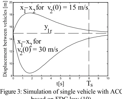
Since u now appears on the RHS, (16) will _i be used to form the FDC. This is practicable since all the other variables on the RHS are either direct measurements available on vehicle, i, or may be obtained by software differentiation of these measurements, except for v , which may estimated using _di an observer. The desired closed-loop dynamics has to be of second order since the plant rank is 2 with respect to the controlled output, y_1i, according to (16). This will be chosen as critically damped with a settling time, of T_s seconds (3% criterion). Using the Dodds settling time formula (Vittek and

Dodds, 2003), the poles of the closed-loop system are set to

(

)

1,2 s

s = −1.5 1 n T+ (17)

where n is the order. This yields the following desired closed-loop differential equation:

(

)

1i 2 1ir 1i 1i s s

81 9

y y y y

T T

= − −

&& & (18)

where y_12r is the reference input, which in this case is the demanded distance between the vehicles. The FDC law is then obtained by equating the RHSs of (18) and (16) and solving for u : _i

(

)

i

M 2i i 2 1i 1ir 1i 2i 3i di L

s

s 1i

y

81 9

u y y y y y Cv

T

T y

= − + _& +_& +_& −

(19)

[image:5.595.312.516.401.566.2]

Figure 3 shows a simulation equivalent to that of Figure 2 but with (19) and T_s=8s.

Figure 3: Simulation of single vehicle with ACC based on FDC law (19).

As it stands, the FDC ACC control law would take control regardless of the distance separating the vehicles. A more practicable ACC system, however, would only take control if the vehicle approached relatively closely to the vehicle in front and allowed the driver the complete freedom she/he should have at relatively large distances. The ability of FDC to yield a nonlinear desired closed-loop dynamics renders this possible. ‘Relatively close’ will be defined as

0 1 2 3 4 5 6 7 8 9 10

8 10 12 14 16 18 20

t[s]

D

is

pl

acemen

t b

et

w

ee

n v

eh

icles

[

m

]

x x for v (0) = 15 m/s

Ts 1

1 2

2 2

−

1r 2

y

x x for v (0) = 30 m/s

1i 1c

y <y , where y_1c is the control transition distance, which is chosen as 20 m for the simulations to follow. At large distances, the ‘closed-loop’ dynamics should be the same as the vehicle without ACC, i.e., given by (16) with u_i =0 and should be given by (18) at relatively small distances. To avoid impulsive accelerator or brake action when (18) comes into play, the transition between (16) (with u_i =0) and (18) should be continuous. Thus, the desired closed-loop dynamics is chosen as follows:

( ) (

)

( )

i

1i 1i 2 1ir 1i 1i s s

M 2i 1i 2i 3i di L

1i

81 9

y y y y y

T T

y

1 y y y C v

y

 

 

= λ − −

 

 

 

 

 

+ − λ_{  } + −



 

&& &

& &

(20)

where λ

( )

y_1i is the control transition function

satisfying:

( )

( )

( )

lim 1i 1i 1c lim 1i 1i

y 0 y 1

y 0.5

y y 0



→ λ =



λ =



 _{→ ∞ λ =}



. (21)

The control transition function has a sharpness parameter, δ, that can be adjusted, and is based

on Ambrosino’s smooth approximation to the signum function used to eliminate control chatter in sliding mode control (Utkin, 1992):

( )

1 1i 1c

1i 2 1i 1c y y y 1 y y  ₋   

λ = −

− + δ

 

 

(22)

Figure 4 shows a sketch of this function:

Figure 4: Control transition function.

The FDC design will now be carried out using (29) for the desired closed-loop dynamics. Hence equating the RHSs of (29) and (25) and solving the resulting equation for u yields: _i

( )

(

)

i

1i 1ir 1i 2

s s

i 1i

M 2i 2i 3i di L 1i

81 9

y y y

T T

u y _y

y y Cv

y

 _{− +} 

 

 

=λ _{ }

[image:6.595.312.500.289.446.2]

+ + −       & & & (23)

Figure 5 shows a simulation equivalent to that of Figure 3.

Figure 5: Simulation of single vehicle with ACC based on FDC law (23) with δ =1m.

In this case, it is evident that when the closing velocity is negative, i.e., vehicle 1 is pulling away from vehicle 2, the ACC becomes inactive allowing the driver complete freedom, but for a relatively large positive closing velocity, the ACC brings vehicle 2 under control in a non-oscillatory fashion to reach the prescribed following distance of y_1r =15m.

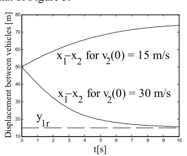
Now 20 vehicles following one another without ACC are simulated in Figure 6. Initially, the vehicles are travelling at 20 m/s wit a constant spacing of 15 m. After 2 seconds the lead vehicle 1 brakes at -4 m/s/s for 2 [s] and then continues at a constant speed of 16 m/s. All vehicles have identical mathematical models to that of the previous simulations. The oscillation build-up and the consequent onset of congestion is immediately evident.

0 1 2 3 4 5 6 7 8 9 10

10 20 30 40 50 60 70 80 t[s] D is place men t b et w een v eh icl es [ m ]

x x for v (0) = 15 m/s

y

2 2 1−

1

x x for v (0) = 30 m/s− ₂

2

1r

1c

y y_1i

( )

y1i

λ 0 1 0.5 0.75 0.25 δ δ 0

[image:7.595.78.253.113.392.2]

Figure 6: Simulation of a 20 vehicle train without ACC.

Figure 7: Simulation of a 20 vehicle train with ACC based on FDC law (23) with δ =1m.

Figure 7 shows a repeat of the simulation of Figure 6 with the same initial conditions and braking of the lead vehicle but with al the nineteen following vehicles fitted with ACC based on FDC law (23). It is clear that the wave build-up and subsequent congestion has been eliminated.

8. Conclusions and Recommendations

A general model-based control method, forced dynamic control, has been produced that is applicable to both linear and nonlinear plants and that may be designed to yield a chosen linear or nonlinear closed-loop dynamic response to the reference inputs. An initial investigation of the application of FDC to improve traffic dynamics has been studied by simulation and shows sufficient promise to warrant further work. Other traffic dynamic models than the GHR model should be considered and the application of forced dynamic control with various prescribed closed loop dynamics, particularly taking into account the effects on the feel of the vehicle to the driver.

9. References

Dodds, S.J. and Gu, X. Y., “Forced Dynamic Control”, AICE2005 International Conference, Accra, Ghana, August, 2005

Isidori, A., Nonlinear Control Systems, 3rd Edition, Springer-Verlag, 1995.

Ossen and Hoogendoorn, “Car-Following Behaviour Analysis from Microscopic Trajectory Data”, Study Report: Delft University of Technology, NL, 2004.

Utkin, V. I., Sliding Modes in Control and Optimisation, Springer Verlag, 1992.

Vittek, J. and Dodds, S. J., Forced Dynamics Control of Electric Drives, University of Zilina Press, 2003, ISBN 80-8070-087-7.

0 10 20 30 40 50 60 70 80

0 50 100 150 200 250

300 Bottom graph: Vehicle 2; Top graph: Vehicle 20.

t[s]

Di

st

an

ce

to

le

ad

v

eh

icl

e [

m

]

0 10 20 30 40 50 60 70 80

15 16 17 18 19 20 21

t[s]

Ve

hi

cl

e ab

so

lu

te

v

el

oci

ti

es

[m

/s

]

Lead vehicle Vehicle 20

0 10 20 30 40 50 60 70 80

0 50 100 150 200 250 300

t[s]

D

is

ta

nc

e t

o l

ead

v

eh

icl

e [

m

]

Vehicle 20 to lead vehicle

Vehicle 2 to lead vehicle

0 10 20 30 40 50 60 70 80

11 12 13 14 15 16 17 18 19 20

t[s]

V

eh

ic

le

a

bs

olu

te

v

elo

citie

s [

m

/s

]

Lead vehicle

[image:7.595.77.254.411.692.2]