Yardstick competition: a spatial voting model approach

Munich Personal RePEc Archive

Yardstick competition: a spatial voting

model approach

Canegrati, Emanuele

April 2006

Online at

https://mpra.ub.uni-muenchen.de/1017/

Yardstick Competition in Presence of Shocks: A

Spatial Voting Model Approach

Emanuele Canegrati

October 5, 2006

1

Abstract

I analyse a yardstick competition game using a spatial voting model, where voters vote for a candidate according to the distance between their Ideal Point and the policy selected by a candidate. The policy which is closest to a voter’s IP provides the voter with a higher util-ity so that minimizing the distance means maximising the utilutil-ity. I demonstrate that in the presence of asymmetrical information the ex-istence of yardstick competition entails a selection device but not a discipline device, suggesting the existence of a trade off between these two goals. In the second part, I analyse an economic environment characterised by the presence of shocks, whose sign and magnitude are a private information of incumbents. This time, the introduction of yardstick competition acts both as a selection and a discipline device.

1_{DEFAP - Universita’ Cattolica del Sacro Cuore - Milan; e-mail address:}

1

Introduction

enforces more the selection than the discipline effect. On the negative side are also Bordignon et al. ([7]), which used a theoretical tax-setting model which demonstrates how the yardstick competition may induce more pool-ing or separatpool-ing behavior among different types of government, dependpool-ing on model parameters.

The goal of this paper is twofold: first of all, it analyses a typical yardstick competition game from a new perspective represented by a spatial voting model. Spatial voting models have been deeply studied in the literature from a theoretical perspective2, but strange enough these studies still have not found many applications in real economic problems. One of the main assumptions of a spatial voting model is that individuals have an Ideal Point (IP) in a multi issue space, which represents the point where they get the maximum satisfaction. As a consequence, it is natural to think they vote for a candidate who sets the closest policy to their IP. Roughly speaking, they vote according to the distance between the ideal policy they have in mind and the real policy a government sets. This conjecture is subtle. Usually, in Bayesian games, we have good and bad types of individuals. The concept of “good”or “bad”is a-priori determined. A good type is who pursues the society’s interest and the bad is who pursues its own interests. In a spatial voting model the concept of “goodness”or “badness”is more relative. Since the exclusive criterion agents use to evaluate a politician is represented by thedistance, they perceive a candidate as good if that candidate chooses a closer policy to their IP than another candidate, who is automatically per-ceived as bad. Thus, voters tend to evaluate candidates according to a very egoistic criterium: they only vote candidates who they feel very close to their needs. This is not far from what happens in the real world. Everyone of us casts his vote evaluating the “distance”he feels between his position and candidate’s position. Notice that the distance perceived may be due to several reasons: one may decide to vote for a candidate because he evaluates that he will provide him more money transfers or may vote for it because he feels that theideological distance is small. A voter may adopt different cri-teria of evaluation, but the important thing here is that he is always able to translate his evaluation in a metric distance, and vote for a candidate whose distance from his IP is the minimum. Mathematically speaking, we are solv-ing a duality problem: minimissolv-ing the distance between the voter’s IP and the candidate’s policy means maximising the voter’s utility. Secondly, refer-ring to the resolution of the yardstick game, it will be demonstrated that in a situation where voters are not able to evaluate the type of incumbent and the type of shock which affects the economy but they perfectly evaluate the outcome of policies of different jurisdictions, equilibria may be both pooling and separating. Thus, the yardstick competition may exacerbate the

will-2_{the literature on spatial voting models is huge: see Hinich & Ordeshook, 1970 ([13]),}

ingness of bad candidates of immediately separate from good candidates. As a consequence the yardstick competition contributes to select good and bad politicians but also acts an incentive device to promote efficiency. The paper is organized as follows: section 1 briefly introduce the voting model litera-ture, section 2 analyses the general features of the model, section 3 analyses a model characterized by complete information, section 4 and 5 analyses the same model in which there exists asymmetrical information both in the absence and in the presence of yardstick competition, section 6 and 7 adds the presence of shocks in the model, section 8 concludes. Finally, Appendix A provides a technical discussion of the most important lemmas of spatial voting models and Appendix B provides an analysis of the multivariate case.

2

The model

2.1 Candidates

I consider a two-period model with three political candidates D,R and W, where D stands for Democratic, R for Republican and W for Welfaristic. On each party I attached a political label, which I assume is exogenously taken at the beginning of the electoral campaign. For instance, we may think about the most familiar labeling system in the U.S., where candidates are located in a left-right or liberal-conservative scale. In our model we assume that candidate R is labeled as “conservative”and that, in a very simplified vision, it is supported by voters who get higher utility in the taxation of labor rather than capital. Otherwise, the candidate D is labeled as “liberal”and he supports voters who get higher utility in the taxation of capital rather than labor. Thus, the space of candidates is given by ΘC _{= {D, R, W}.}

Furthermore candidate D may be agood type or abad type and so may be candidate R. Thus, the space of type is ΘG = nθDg, θDb, θRg, θRbo. Each candidate may play only 4 policies: two populistic policies (the right-wing populistic policy aR and the left-wing populistic policy aD), which provide more welfare to oriented voters, a welfaristic policy aW, which is neutral and a bad policyabp which enables the government to subtract rents to the society’s welfare.

2.1.1 Candidate’s preferences

Each candidate has the following preferences ordering: Candidate D good type: aD ≻aW ≻aR≻abp

Candidate D bad type: abp ≻aD ≻aW ≻aR

Candidate R good type: aR≻aW ≻aD ≻abp

Candidate R bad type: abp≻aR≻aW ≻aD

that ax ay ⇔ r(ax) ≥r(ay). Thus, in utility terms, candidate’s prefer-ences may be represented in the following manner:

Candidate D good type: r(aD)> r(aW)>

=0

z }| {

r(aR)> r(abp)

Candidate D bad type: r(abp)> r(aD)>

=0

z }| {

r(aW)> r(aR)

Candidate R good type: r(aR)> r(aW)>

=0

z }| {

r(aD)> r(abp)

Candidate R bad type: r(abp)> r(aR)>

=0

z }| {

r(aW)> r(aD)

To facilitate calculations, I assume the existence of a strict preferences or-dering (the inequality is strict) and that the third term of the oror-dering is normalized to zero.

2.2 Voters

I suppose the existence of a population of voters, portioned in three equal groups (i.e. 1 voter per group): the welfarist voters, who are those who have not any particular preference for a candidate, candidate D-oriented voters, who support the Democratic Party and candidate R-oriented voters, who support the Republican Party.

2.2.1 Voter’s preferences

Each voter has the following preferences ordering: D-oriented Voter: aD ≻aW ≻aR≻abp

R-oriented Voter: aR≻aW ≻aD ≻abp

Welfarist Voter: aW ≻aD∨aR≻abp

Voters observe candidate policies and cast their vote for the candidate who has selected the nearest policy to their IP. In Appendix A I provide a tech-nical explanation of the mechanism adopted by voters to select which is the candidate who provide them the highest utility.

3

A complete information case

take place. Voters perfectly recognize the type of candidate, so that parties cannot exploit any information advantage, and they cast their vote to the party which chooses a policy vector closer to their IPs. [FIGURE 1 HERE] Figure 1 shows the IP of each voter (black singletons), while concentric cir-cles represents voter’s indifference curves. The smaller the circle, the nearer the policy chosen by a candidate to the voter’s IP and the higher the utility the voter gets. Voters who support the Republican party have an ideal point such as R, where the tax rate on capital is equal to zero and the tax rate on labor is equal to one. Symmetrically, voters who support the Democratic party have an ideal point such as D, where the tax rate on labor is equal to zero and the tax rate on capital in equal to one. In the middle of the space, on W, are located welfaristic voters, that may be intended as “super-rational”voters who do not have any particular preference toward one of the two candidates.

Circles correctly represent the voters’ utility preferences only if voters as-sign exactly the same weight to every dimension of the policy space. If not, the utility preference is given by a non circular structure, that indi-cates that the decrease in utility is not the same in every dimension. In my example we have a policy vector given bya={τl, τk} in the Cartesian

spaceτl×τk; we can represent voters’ preferences with circles if and only if: ∂U(τl,τk)

∂τl =

∂U(τl,τk)

∂τk ; otherwise, if

∂U(τl,τk)

∂τl 6=

∂U(τl,τk)

∂τk voters’ preferences are

represented by ellipses, where the longer axis refers to that dimension which shows the higher decrease in the utility with respect to the other dimension, once we move away from the IP. Figure 2 sketches a typical situation where the decrease in utility is not the same in every direction. Furthermore, the rotation of the major and the minor axis of the elliptical contours of each citizen’s loss function may be represented by a matrix of coefficients. If this matrix is equal for every voter, then we are in the “common orienta-tion”case, and the ellipses have the same rotation axis.

[FIGURE 2 HERE]

Finally, voters’ preferences are uniformly distributed (in a discrete case), while they are represented by a density function, say f(x), which is radial symmetric3 and unimodal (in a continuous case). Figure 3 shows the candi-dates’ IPs. Initially, we assume that candidate IPs must only stand over the budget constraint line; this assumption may be realistic as candidates are Welfaristic with a slight preference toward one of the two ideological voters. Thus, candidates can only choose a policy which stands over the budget constraint line.

[FIGURE 3 HERE]

Furthermore, I assume that the party which gets the majority of votes win the elections; in the case of a tie a coin is tossed as to decide which party will take power. Finally the utility that voters get in the second period of

3_{that isf(x) =f(}

the game is discounted by a discount factorβ ∈[0,1].

Proposition 1 In an economy with a finite number of identical voters the two parties choose the vector of policies which exactly coincides with the Welfarist voter’s IP, if and only if they discount the future sufficiently little; otherwise, they prefer to locate exactly on their preferred IPs.

Proof: In the second period of the game, once the elections have taken place, the elected candidate chooses the policy which stands on its IP (aD

for party D andaRfor party R). Otherwise, in the first period, parties choose the policy which maximizes the expected utility over the two periods. Since the two parties can only play either a populistic policy or a welfaristic policy, we can depict this situation of strategic interaction between the two parties by the meaning of the following game:

aR _aW

aD _r(aD_{) +}1

2βr(aD);r(aR) +12r(aR) r(aD);r(aW) +βr(aR)

aW _r(aW_{) +βr(a}D_);r(aR_{) r(a}W_{) +}1

2βr(aD);r(aW) +12βr(aB)

Rows show policies played by party D, while columns policies played by party R and the four boxes show payoffs of the game with the two parties’ expected utilities. If party R plays aR Party D plays aD if and only if r(aD|aR) > r(aW|aR). This happens whenr(aD) +1₂βr(aD)> r(aW) +βr(aD) or when

β ∈ [0,2(1− a_aWD)). If party R plays aW Party D plays aD if and only if

r(aD|aW) > r(aW|aW). This happens when r(aD) > r(aW) + 1₂βr(aD) or

β∈[0,2(1−a_aWD)). The same holds for party R.

Then, we may distinguish three cases:

1. whenβ ∈[0,2(1−a_aWD)) the only one Nash equilibrium is one such that

the two parties play a populistic strategy which enables them to get the maximum utility; elections’ outcome is a tie and a coin is tossed to decide which candidate will take power in the second period.

2. when β ∈ (2(1− a_aWD),1] the only one Nash equilibrium is one such

that the two parties play the welfaristic policy which coincides with the welfaristic voter’s IP; elections’ outcome is again a tie.

3. when β = 2(1− a_aWD) the two parties are indifferent to play either aD

oraW and then infinite equilibria in mixed strategies arise.

4

A game with incomplete information and

ab-sence of shocks

as ΘG₌n_θDg_{, θ}Db_{, θ}Rg_{, θ}Rbo_{, where g denotes the good type andb the bad}

type. Furthermore, I introduce an asymmetry in information between the two parties, such that the incumbent does not know whether it is challenging a good or a bad opponent; it only knows that there exists ana priori prob-ability equal toq that the challenger is a good type and a probability equal to 1 - q that the challenger is a bad type. The distribution of probability is common knowledge between candidates and voters, in the sense that also voters know the existence of this a-priori probability that candidate is good (this probability may be see as the reputation of the candidate). Figure 4 shows the policy Cartesian spaceτl×τk, which can be normalized to 1×1.

The straight line represents the Government budget constraint being equal to zero. With respect to the previous case, two additional IP point (GDb and GRb) have been added and they represent the IP of bad Governments (party D and R respectively). These two points represent a location where Governments can get a rent which is equal to the distance from any policy which stands in the North-East triangle above the budget constraint line and the budget constraint line. The longer this distance, the higher the rent subtracted by the Government.

[FIGURE 4 HERE]

I study two cases where the incumbent may be either a good or a bad type. In the first I study a case where the incumbent may face a good challenger which is “super-welfarist ”in a sense that he always plays strategy aW or a bad Government who can only play strategy abp. Thus, the game can be formalized in the following structure:

ΘC ={D, R, W}

ΘG =nθDg, θDb, θRg, θRbo

AI =AD =naD, aR, aW, abpo⊆E₂

AGg =ARg =naWo⊆E2

AGb =ARb =nabpo⊆E2

Pr(θR=θRg) =q

Pr(θR=θRb) = 1−q

ΘC _{={D, R, W}}

ΘG ₌n_θDg_{, θ}Db_{, θ}Rg_{, θ}Rbo

AI =AD =naD, aR, aW, abpo⊆E2

AGg =ARg =naRo⊆E2

AGb =ARb =nabpo⊆E2

Pr(θR=θRg) =q

Pr(θR=θRb) = 1−q

Proposition 2 If the incumbent is a good type, he plays the populistic strat-egyaD ifq ∈[0,_βr(2_aD₎(r(aD)−r(aW))), whilst he plays the welfaristic

strat-egy aW if q∈(_βr(2_aD₎(r(aD)−r(aW)),1].

Proof: EU(aD) =r(aD) +β(1−q)r(aD) is always greater than EU(aR) =

r(aR) +β(1−q)r(aR) and thanEU(abp) =r(abp) +1₂β(1−q)r(aD), whilst it is greater than EU(aW) = r(aW) + 1₂βqr(aD) +β(1−q)r(aD) for q ∈

[0,_βr(2_aD₎(r(aD)−r(aW)))4.

This result can be interpreted as follows: if the probability to face a good challenger is sufficiently small, the incumbent has a great opportunity to play a policy which stays on his IP. Otherwise, if the probability to face a good challenger is high, the incumbent realizes that playing his preferred policy would not be sufficiently safe to assure the re-election and then he prefers to play a welfaristic policy to get the welfaristic citizens’ votes.

Proposition 3 If the incumbent is a bad type, he plays the populistic strat-egy aD if q∈[0,_βr(2_abp₎(r(aD)−r(abp) +1₂βr(abp))), whilst he plays the bad

policyabp if q ∈(_βr(2_abp₎(r(aD)−r(abp) + 1₂βr(abp)),1]

Proof: EU(aD) =r(aD) +β(1−q)r(abp) is always greater thanEU(aR) =

r(aR) +β(1−q)r(abp) and EU(abp) = r(abp) + 1₂β(1−q)r(abp) is always greater than EU(aW) = r(aW) + 1₂βqr(abp) +β(1−q)r(abp). EU(aD) is greater thanEU(abp) for q∈[0,_βr(2_abp₎(r(aD)−r(abp) +1₂βr(abp))).

The result says that if the probability that the incumbent faces a good challenger is sufficiently low he plays the populistic strategy, since the elec-torate is always able to see the bad strategy undertaken by the party (bad type) and reelect the incumbent, since it is not able to evaluate whether the type is good or bad. Otherwise, if the probability to face a good challenger is high, the bad incumbent realizes that it becomes too costly mimicking a good type (which would entail a pooling equilibrium) and so he plays the bad policy even though he knows that he will lose the elections. As a con-sequence a separating equilibrium arises. Analyse now the situation where the government (good type) is committed to play the populistic strategy.

Proposition 4 If the incumbent is a good type, he plays the populistic strat-egyaD ifq ∈[0,_βr(2_aD₎(r(aD)−r(aW))), whilst he plays the welfaristic

strat-egy aW if q∈(_βr(2_aD₎(r(aD)−r(aW)),1]

4_{A note: In all the proofs, the expressionalways greater which refers to the expected}

Proof: same as before.

Proposition 5 If the incumbent is a bad type, he plays the populistic strat-egy aD if q∈[0,_βr(2_abp₎(r(aD)−r(abp) +1₂βr(abp))), whilst he plays the bad

policyabp if q ∈(_βr(2_abp₎(r(aD)−r(abp) + 1₂βr(abp)),1]

Proof: same as before.

5

A case of yardstick competition

I introduce now the yardstick competition framework. The main goal is to verify how the introduction of another jurisdiction may act as a discipline device for candidates. I suppose that domestic voters are able to update their beliefs about the domestic government by comparing the policy it un-dertakes with that undertaken by the foreigner jurisdiction. I demonstrate that, due to this comparison, the bad domestic candidate refrains himself to mimic the good type, since the mimicking strategy would become too costly for him. As a consequence, we expect a reinforcement of separating equilibria and a weakening of pooling equilibria. I consider at first a foreign government which can be either a good or a bad type. If he is good, he plays a welfaristic strategyaW F, whilst if he is bad, he plays a bad policy strat-egyabpF. Later on, I will consider a good government committed to play a populistic strategyaRF, instead of playingaW F, whilst the bad government plays the bad policy strategyabpF. Thus, the game can be formalized in the following terms:

ΘC ₌n_{D, R, W, D}F_{, R}F_{, W}Fo

ΘG =nθDg, θDb, θRg, θRb, θDgF, θDbF, θRgF, θRbFo

AI =AD =naD, aR, aW, abpo⊆E2

AIF =AD =naDF, aRF, aW F, abpFo⊆E2

AGg =ARg =naWo⊆E2

AGb =ARb =nabpo⊆E2

AGbF =ARbF =nabpFo⊆E2

Pr(θR=θRg) =q

Pr(θR=θRb) = 1−q

Pr(θRF =θRgF) =x

Pr(θRF =θRbF) = 1−x

Again I find perfect Bayesian equilibria of the game.

Proposition 6 If the incumbent is a good type, he plays the populistic policy

aD if q ∈ [0,_βr(2_aD₎(r(aD)−r(aW))), whilst he plays the welfaristic policy

aW if q∈(_βr(2_aD₎(r(aD)−r(aW)),1].

Proof: EU(aD) = r(aD) + β(1−q)(1−x)r(aD) is always greater than

EU(aR) =r(aR) +β(1−q)(1−x)r(aD) andEU(aD) is always greater than

EU(abp) =r(aW) +1₂β(1−q)(1−x)r(aD). EU(aD) is greater thanEU(aW) forq∈[0,_βr(2_aD₎(r(aD)−r(aW))).

Proposition 7 If the incumbent is a bad type, he plays the populistic policy

aD if q∈[0,_βr(abp2_)(1−x)(r(aD)−r(abp) + 1₂βr(abp)(1−x))), whilst he plays

the bad policy abp if q∈(_βr(abp2_)(1−x)(r(aD)−r(abp) +1₂βr(abp)(1−x)),1].

Proof: EU(aD) = r(aD) + β(1−q)(1−x)r(aD) is always greater than

EU(aR) =r(aR) +β(1−q)(1−x)r(aD) andEU(aD) is always greater than

EU(abp) =r(aW) +1₂β(1−q)(1−x)r(aD). EU(aD) is greater thanEU(aW) forq∈[0,_βr(2_aD₎(r(aD)−r(aW))).

These results show how the probability to face a foreigner good type directly enters into the equilibrium intervals, meaning that the domestic incument changes the policies played not only taking into account the probability to face a good domestic challenger, but also taking into account the probability to find a good foreign Government.

Suppose now to slightly change the previous game, such as the domestic government (good type) plays the populistic policy aR instead of the wel-faristic policyaW. The game becomes:

ΘC ₌n_{D, R, W, D}F_{, R}F_{, W}Fo

ΘG =nθDg, θDb, θRg, θRb, θDgF, θDbF, θRgF, θRbFo

AIF =AD =naDF, aRF, aW F, abpFo⊆E2

AGg =ARg =naRo⊆E2

AGb =ARb =nabpo⊆E2

AGgF =ARgF =naW Fo⊆E2

AGbF =ARbF =naRbFo⊆E₂

Pr(θR=θRg) =q

Pr(θR=θRb) = 1−q

Pr(θRF =θRgF) =x

Pr(θRF =θRbF) = 1−x

Proposition 8 If the incumbent is a good type, he plays the populistic strat-egy aD if q ∈ [0, 1r(aW)+(xβ−1)r(aD)

2βr(aD)−βr(aD)(1−x)

), whilst he plays the welfaristic policy

aW if q∈(1r(aW)+(xβ−1)r(aD) 2βr(aD)−βr(aD)(1−x)

),1].

Proof: EU(aD) =r(aD) +1₂βqr(aD) +β(1−q)r(aD) is always greater than

EU(aR) =r(aR) +1₂βqr(aD) +β(1−q)r(aD) andEU(aD) is always greater than EU(abp) = r(abp) + 1₂β(1−q)(1−x)r(aD). EU(aD) is greater than

EU(aW) for q ∈[0, 1r(aW)+(xβ−1)r(aD) 2βr(aD)−βr(aD)(1−x)

).

Proposition 9 If the incumbent is a bad type, he plays the populistic

strat-egyaD ifq ∈[0,(1+β)r(a

D_)−r(abp₎₋1 2βr(a

D_)(1−x)

1 2βr(aDx)

), whilst he plays the bad policy

abp if q∈((1+β)r(aD)−r(abp)−12βr(a

D_)(1−x)

1 2xβr(aD)

),1].

Proof: EU(aD) =r(aD) +βqr(aD) +β(1−q)r(aD) is always greater than

EU(aR) =r(aR) +βqr(aD) +β(1−q)r(aD) and EU(aD) is always greater than EU(abp) = r(abp) + 1₂β(1−q)(1−x)r(aD). EU(aD) is greater than

EU(aW) for q ∈[0,(1+β)r(aD)−r(abp)−12βr(aD)(1−x) 1

2xβr(aD)

).

in the absence of yardstick competition case, which suggests that separating equilibria are more likely to happen. Furthermore, this suggests the impor-tant role played by the yardstick competition as aself-selection device. Once voters have the possibility to compare domestic and foreign policies, bad can-didates realize that it becomes more costly to mimic the good governments and then prefer to immediately separate. This is a positive result because it shows as bad candidates are more likely to be recognized and thrown out of the office. Otherwise, the yardstick competition fails to achieve the disci-pline device goal. In fact, bad politicians are not forced to behave efficiently and thus this entails that voters are worse off. In this economic environment, the conclusion about the role of the yardstick competition is that there ex-ists a trade-off between theself-selection goal and thediscipline devicegoal. Since I supposed the existence of perfect correlation among economies, my results support the theory by Bordignon et al. ([7]) which affirms that “the larger is the degree of correlation between economies, the more the citizen learns by observing the fiscal choices in the other jurisdiction, and the more difficult it is for the bad politician to escape detection when cheating ”.

environment eq.strategy/intervals

1/n/g aD_/[0, 2

βr(aD₎(r(aD)−r(aW))) aW_/( 2

βr(aD₎(r(aD)−r(aW)),1]

1/y/g aD_/[0, 2

βr(aD₎(r(aD)−r(aW))) aW_/( 2

βr(aD₎(r(aD)−r(aW)),1]

1/n/b aD_/[0, 2

βr(abp₎(r(aD)−r(abp) +1₂βr(abp))) abp_/( 2

βr(abp₎(r(aD)−r(abp) +12βr(abp)),1]

1/y/b aD_/[0, 2

βr(abp₎₍₁₋x)(r(a

D_)−r(abp_{) +}1 2βr(a

bp_)(1−x)))

abp_/( 2

βr(abp_)(1−x)(r(aD)−r(abp) +12βr(abp)(1−x)),1]

2/n/g aD_/[0, 2

βr(aD₎(r(a

D_)−r(aW₎₎₎

aW_/( 2

βr(aD₎(r(aD)−r(aW)),1]

2/y/g aD_/[0,−r(aD)+r(aW)+xβr(aD)

1

2βr(aD)−βr(aD)(1−x)

)

aW_/(−r(aD)+r(aW)+xβr(aD)

1

2βr(aD)−βr(aD)(1−x)

,1] 2/n/b aD_/[0, 2

βr(abp₎(r(a

D_)−r(abp_{) +}1 2βr(a

bp₎₎₎

abp_/( 2

βr(abp₎(r(aD)−r(abp) +1₂βr(abp)),1]

2/y/b aD_/[0,(1+β)r(aD)−r(abp)−12βr(a

D_)(1−x)

1 2βr(aD)x

)

abp_/((1+β)r(aD)−r(abp)−12βr(a

D_)(1−x)

1 2βr(aD)x

),1]

Table 1 _{- equilibrium strategy - Legend: (1) refers to the case where the good government}

6

A game with incomplete information and

pres-ence of shocks

In this second part, I allow for the possibility that some shocks may occur in the economy; these shocks may be seen as all of those exogenous events which may increase (or decrease) efficiency in the production of public goods. Shocks may be either positive (P) or negative (N); if a shock is positive, then the efficiency in the production increases whilst if the shock is negative the efficiency decreases. An increase in efficiency may be seen as the possibility to produce the same amount of good at a lower cost, or to produce an higher amount of that good at the same cost. The cost of production is borne by taxation and thus, citizens are better off when a shock is positive, since they pay less taxes. An important assumption here is that the sign and the magnitude of the shock is a private information of candidates, which perfectly observe whether these are positive or negative. Otherwise, voters only perceive the existence of shocks but are not able to measure neither the magnitude nor the sign. Thus, at the beginning of the game, Nature choose both the type of candidates and the type of shock. Candidates observe Nature’s choice and then announce (and commit) to a policy which depends on the type of shock, that is a(ǫ); voters observe candidate’s policies and vote for the candidate who chooses the nearest policy with respect to their IP.

6.1 Positive shock

Suppose at first that the economy is affected by a positive shock. I write the preferences for every government type.

θDg:r(aD(ǫP))> r(aW(ǫP))> r(aR(ǫP))>0> r(aD(ǫN))> r(aW(ǫN))> r(aR(ǫN))> r(abp)

θDb:r(abp)> r(aD(ǫN))> r(aW(ǫN))> r(aR(ǫN))>0> r(aD(ǫP))> r(aW(ǫP))> r(aR(ǫP))

θRg:r(aR(ǫP))> r(aW(ǫP))> r(aD(ǫP))>0> r(aR(ǫN))> r(aW(ǫN))> r(aD(ǫN))> r(abp)

θRb_:r(abp_{)> r(a}R_(ǫN_{))> r(a}W_(ǫN_{))> r(a}D_(ǫN_{))>0> r(a}R_(ǫP_{))> r(a}W_(ǫP_{))> r(a}D_(ǫP₎₎

[FIGURE 5 HERE]

Figure 5 shows the IP of each government type when the shock is positive. Line BC indicates the locus where the budget constraint is equal to zero. This is a private information of the government. Notice that the welfaristic strategy W and the strategy played by government good type GDg and

Proposition 10 If the incumbent is a good type, he plays the populistic strategyaD(ǫP)ifq ∈[0,_βr(aD2_(ǫP₎₎(r(aD(ǫP))−r(aW(ǫP)))), whilst he plays

the welfaristic policy aW(ǫP) if q∈(_βr(aD2_(ǫP₎₎(r(aD(ǫP))−r(aW(ǫP))),1].

Proof: The bad policy, policies which are a function of the negative shock and policies which stand on the B’s IP are strictly dominated by aD(ǫP) and aW(ǫP).

Notice here that a government (good type) always chooses a policy which stands over the budget constraint line, even though the exact location over this line aD(ǫP) or aW(ǫP) changes with respect to probability intervals.

Proposition 11 If the incumbent is a bad type, he plays the populistic strat-egy aD(ǫN) if q ∈ [0,_βr(abp2_(ǫP₎₎(r(aD(ǫN))−r(abp) + 1₂βr(abp))), whilst he

plays the bad policy abp if q ∈(_βr(abp2_(ǫP₎₎(r(aD(ǫN))−r(abp) +1₂βr(abp)),1]

Proof: the bad policy and the populistic strategy strictly dominates all the other strategies.

Notice in this case how a bad incumbent is willing to make voters believe that a shock is negative, since if they believed so, he would be able to adopt a policy which would stand at a closer point to his IP.

6.2 Negative shock

Suppose now that the economy is affected by a negative shock and write again the preferences for every government type.

θDg:r(aD(ǫN))> r(aW(ǫN))> r(aR(ǫN))>0> r(aD(ǫP))> r(aW(ǫP))> r(aR(ǫP))> r(abp)

θDb_:r(abp_{)> r(a}D_(ǫN_{))> r(a}W_(ǫN_{))> r(a}R_(ǫN_{))>0> r(a}D_(ǫP_{))> r(a}W_(ǫP_{))> r(a}R_(ǫP₎₎

θRg_:r(aR_(ǫN_{))> r(a}W_(ǫN_{))> r(a}D_(ǫN_{))>0> r(a}R_(ǫP_{))> r(a}W_(ǫP_{))> r(a}D_(ǫP_{))> r(a}bp₎

θRb_:r(abp_{)> r(a}R_(ǫN_{))> r(a}W_(ǫN_{))> r(a}D_(ǫN_{))>0> r(a}R_(ǫP_{))> r(a}W_(ǫP_{))> r(a}D_(ǫP₎₎

[FIGURE 6 HERE] Figure 6 shows the Ideal Point of each government type when the shock is negative. Line BC indicates the locus where the budget constraint is equal to zero. Unlike the previous case, this time the budget constraint stand north-eastward; this means that is more costly for Government to produce public goods and it needs a higher level of taxation. Notice also how the welfaristic strategy W does not stand over the same line where the strategy played by government good type GDg and GRg

Proposition 12 If the incumbent is a good type, he plays the populistic policyaD(ǫN) ifq ∈[0,_βr(aD2_(ǫN₎₎(r(aD(ǫN))−r(aW(ǫN)))), whilst he plays

the welfaristic policy aW(ǫP) if q∈(_βr(aD2_(ǫN₎₎(r(aD(ǫN))−r(aW(ǫN))),1].

Proof: same as for the positive shock.

Proposition 13 If the incumbent is a bad type, he plays the bad policy abp

ifq ∈[0, 2

βr(abp₎(r(abp)−r(aR(ǫN))−1₂βr(abp))), whilst he plays the populistic

policyaR(ǫP) if q∈(_βr(2_abp₎(r(abp)−r(aR(ǫN))− 1₂βr(abp)),1].

Proof: same as for the positive shock.

7

A case of yardstick competition with presence

of shocks

I analyse now the case of yardstick competition in the presence of shocks where, once again, shocks may be either positive or negative.

7.1 The shock is positive

I suppose that the domestic good incumbent’s preferred policy is aR(ǫP), whilst the bad incumbent’s preferred policy isabp. Furhermore, the foreign good incumbent’s preferred policy is aW(ǫP).

Proposition 14 If the incumbent is a good type, he chooses the populis-tic policyaD(ǫN) ifq ∈[0,_βr(aD_(ǫP1_))(1−x)(r(aD(ǫP))(xβ−1) +r(aW(ǫP)))),

whilst he chooses the welfaristic policyaW(ǫP)ifq∈(_βr(aD_(ǫ1P_))(1−x)(r(aD(ǫP)(xβ−

1) +r(aW(ǫP))),1].

Proof: same as for the absence of yardstick competition case.

Proposition 15 If the incumbent is a bad type, he chooses the populistic policyaD(ǫN)ifq∈[0,_βr(abp2_)(1−x)(r(aD(ǫN))−r(abp)(1−

β

2(1−x)))), whilst

he chooses the bad policyabp ifq∈(_βr(abp2_)(1−x)(r(aD(ǫN))−r(abp)(1−

β

2(1−

x))),1].

Proof: same as for the absence of yardstick competition case.

7.2 The shock is negative

Proposition 16 If the incumbent is a good type, he chooses the populis-tic policy aD(ǫN) if q ∈ [0,_βr(aD1_(ǫN₎₎(r(aW(ǫN))−r(aD(ǫN)))), whilst he

Proof: same as for the absence of yardstick competition case.

Proposition 17 If the incumbent is a bad type, he chooses the populistic policyaD(ǫN)ifq∈[0, 2

βr(abp_)(1−x)(r(aD(ǫN))−r(abp)(1−

β

2(1−x)))), whilst

he chooses the bad policyabp(ǫP) if q∈(_βr(abp2_)(1−x)(r(aD(ǫN))−r(abp)(1−

β

2(1−x))),1]

Proof: same as for the absence of yardstick competition case.

environment eq.strategy/intervals

1/n/g/p aD_(ǫP_)/[0, 2

βr(aD_(ǫP₎₎(r(aD(ǫP))−r(aW(ǫP)))) aW_(ǫP_)/( 2

βr(aD₍ǫP₎₎(r(a

D_(ǫP_))−r(aW_(ǫP_))),1]

1/n/g/n aD_(ǫN_)/[0, 2

βr(aD_(ǫN₎₎(r(aD(ǫN))−r(aW(ǫN))) aW_(ǫN_)/( 2

βr(aD₍ǫN₎₎(r(a

D_(ǫN_))−r(aW_(ǫN_)),1]

1/n/b/p aD_(ǫN_)/[0, 2

βr(abp₎(r(aD(ǫN))−r(abp) +12βr(abp)))

abp_/( 2

βr(abp₎(r(a

D_(ǫN_))−r(abp_{) +}1 2βr(a

bp_)),1]

1/n/b/n aD_(ǫN_)/[0,2(r(aD_(ǫN_))−r(aW_(ǫN₎₎

βr(abp₎ )))if β >

2(r(abp_)−r(aA_(ǫN₎₎

r(abp₎ aW_(ǫN_)/(2(r(aD_(ǫN_))−r(aW_(ǫN₎₎

βr(abp₎ )),1] abp_/[0,2(r(abp)(1−β2)+r(a

w_(ǫN₎₎₎

βr(abp₎ )if β <

2(r(abp)−r(aA(ǫN))

r(abp₎ aW_(ǫN_)/(2(r(abp)(1−β2)+r(a

w_(ǫN₎₎₎

βr(abp₎ ,1]

1/y/g/p aD_(ǫP_)/[0, 1

βr(aD_(ǫP_))(1−x)(r(aD(ǫP))(xβ−1) +r(aW(ǫP)))) aW_(ǫP_)/( 1

βr(aD_(ǫP_))(1−x)(r(aD(ǫP))(xβ−1) +r(aW(ǫP))),1]

1/y/g/n aD_(ǫN_)/[0, 1

βr(aD_(ǫN₎₎(r(aD(ǫN))−r(aW(ǫN)))) aW_(ǫN_)/( 1

βr(aD_(ǫN₎₎(r(aD(ǫN))−r(aW(ǫN))),1]

1/y/b/p aD_(ǫN_)/[0, 2

βr(abp_)(1−x)(r(aD(ǫN))−r(abp)(1−

β

2(1−x))))

abp_/( 2

βr(abp_)(1−x)(r(aD(ǫN))−r(abp)(1−

β

2(1−x))),1]

1/y/b/n aD_(ǫN_)/[0, 2

βr(abp₎(

1 2βr(a

bp_)−r(abp_{) +r(a}D_(ǫN₎₎₎

abp_/(∗, 2

βr(abp₎(−12βr(abp) +r(abp)−r(aW(ǫN)))

aW_(ǫN_/( 2

βr(abp₎(−

1 2βr(a

bp_{) +r(a}bp_)−r(aW_(ǫN_)),1]

2/n/g/p aD_(ǫP_)/[0, 2

βr(aD_(ǫP₎₎(r(aD(ǫP)) +₂1βr(aD(ǫP))−r(aW(ǫP))) aW_(ǫP_)/( 2

βr(aD₍ǫP₎₎(r(a

D_(ǫP_{)) +}1 2βr(a

D_(ǫP_))−r(aW_(ǫP_)),1]

2/n/g/n aD_(ǫN_)/[0, 1

βr(aD_(ǫN₎₎(r(aD(ǫN))(1 +

β

2)−r(a

W_)(ǫN₎₎₎

aW_(ǫN_/( 1

βr(aD_(ǫN₎₎(r(aD(ǫN))(1 +

β

2)−r(aW)(ǫN)),1]

2/n/b/p aD_(ǫN_)/[0, 2

βr(abp₎(r(a

bp₎₍β

2 −1) +r(a

D_(ǫN₎₎₎

abp_/( 2

βr(abp₎(r(a

bp₎₍β

2 −1) +r(a

D_(ǫN_)),1]

2/n/b/n aD_(ǫN_)/[0, 2

βr(abp₎((12β−1)r(abp) +r(aD(ǫN)))

abp_/(∗∗, 1

βr(abp₎((

1

2β+ 1)r(a

bp_)−r(aW_(ǫN₎₎₎

aW_(ǫN_)/( 1

βr(abp₎((12β+ 1)r(abp)−r(aW(ǫN)),1]

2/y/g/p aD_(ǫP_)/[0, 1

βr(aD₍ǫP₎₎(r(aD(ǫP))−r(aW(ǫP)) +21βr(aD(ǫP)))

aW_(ǫP_)/( 1

βr(aD_(ǫP₎₎(r(aD(ǫP))−r(aW(ǫP)) +1₂βr(aD(ǫP)),1]

2/y/g/n aD_(ǫN_)/[0, 1

βr(aD₍ǫN₎₎₍₁₋x)(r(a

D_(ǫN_))−r(aW_(ǫN_{)) +}1

2βr(aD(ǫN))(1−x))

aW_(ǫN_)/( 1

βr(aD_(ǫN_))(1−x)(r(aD(ǫN))−r(aW(ǫN)) +1₂βr(aD(ǫN))(1−x),1]

2/y/b/p aD_(ǫN_)/[0, 2

βr(abp₎₍₁₋x)(a

D_(ǫN_{) +}1

2βr(abp)(1−x)−r(abp))

abp_/( 2

βr(abp₎₍₁₋x)(a

D_(ǫN_{) +}1 2βr(a

bp_{)(1−x)−r(a}bp_),1]

2/y/b/n aD_(ǫN_)/[0, 2

βr(abp_)(1−x)(12βr(abp)(1−x)−r(abp) +r(aD(ǫN)))

abp_{/(∗ ∗ ∗,} 2

βr(abp₎(−r(a

W_(ǫN_{)) +r(a}bp_{) +}1 2βr(a

bp_)(1−x)))

aW_(ǫN_)/( 2

βr(abp_)(2−x)(−r(aW(ǫN)) +r(abp) +12βr(abp)(1−x)),1]

Table 2_{- equilibrium strategy -Legend: (1) refers to the case where the good government}

is committed to play the welfaristic strategy and (2) where is committed to play the populistic strategy; (n) indicitates the absence of yardstick competition case and (y) the presence of yard-stick competition case and (g) indicates the government good type and (b) the government bad type. (∗) 2

βr(abp₎(12βr(abp)−r(abp) +r(aD(ǫN));(∗∗)βr(2abp₎(12βr(abp)−r(abp) +r(aD(ǫN));(∗ ∗

∗) 2

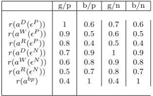
The comparison of results in Table 2 enables us to evaluate the effect of the yardstick competition both as a selective and discipline device. The first observation is that values assumed by parameters of the model (the probability that the foreign government is good and the discount rate) are crucial. Thus, to understand how the introduction of the yardstick competi-tion affects the equilibria, I performed some numerical simulacompeti-tions. Table 3 shows the payoffs for every strategy played and for each type and shock (i.e. b/p stands for bad player and positive shock). Furthermore, Table 4 shows the numerical values which intervals assumes for every equilibrium strategy played in every situation. First of all, notice that when the type is good and the shock is positive the interval where the strategyaD(ǫP) (aW(ǫP)) is played is narrower (broader) in the absence of the yardstick competition, for every value ofβ andx. This means that the yardstick competition forces the good government to play the welfaristic strategy. In this case, it is possible to argue that the introduction of another government acts as a discipline device for the domestic government behavior. The same holds when the shock is negative. When the type is bad, we must distinguish two cases. The first case is when the shock is positive; we are in a situation where the interval where the bad government plays the bad policy is broader than the yardstick competition case, meaning that the existence of a benchmark gov-ernment forces the bad incumbent to separate in the first period and lose elections. This is a case where the yardstick competition acts a selection device. The second case is when the shock is negative. In this situation we must distinguish other two sub-cases, which depend on the parameterβ. In fact, when the discount rate is sufficiently high (β >0.2) the bad incumbent never plays the bad policy, whilst when β is sufficiently low (β <0.2) the bad incumbent replaces the populistic policy previously played, with the bad policy. This is obvious. When the incumbent discount future more, it prefers to immediately gain the first-period rent, whilst if it discounts fu-ture less, it prefers mimicking the good government in the first period to win elections and playing the bad policy only at the second period. The introduction of the yardstick competition produces more difficult results to interpret. In fact, we see that the incumbent may play three equilibrium strategies depending on the parameters of the model.

g/p b/p g/n b/n

r(aD_(ǫP_{)) 1 0.6 0.7 0.6}

r(aW_(ǫP_{)) 0.9 0.5 0.6 0.5}

r(aR_(ǫP_{)) 0.8 0.4 0.5 0.4}

r(aD_(ǫN_{)) 0.7 0.9 1 0.9}

r(aW_(ǫN_{)) 0.6 0.8 0.9 0.8}

r(aR_(ǫN_{)) 0.5 0.7 0.8 0.7}

r(abp_{) 0.4 1 0.4 1}

-environment eq.strategy/intervals

1/n/g/p aD_(ǫP_)/[0,0.2

β )

aW_(ǫP_)/(0.2

β ,1]

1/n/g/n aD_(ǫN_)/[0,0.2

β )

aW_(ǫN_)/(0.2

β ,1]

1/n/b/p aD_(ǫN_)/[0,0.2(0.5β−0.1)

β )

abp_/(0.2(0.5β−0.1)

β ,1]

1/n/b/n aD_(ǫN_)/[0,0.2

β )if β >0.2

aW_(ǫN_)/(0.2

β ,1]

abp_/[0,0.2(1.8−0.5β)

β )if β <0.2

aW_(ǫN_)/(0.2(1.8−0.5β)

β ,1]

1/y/g/p aD_(ǫP_)/[0,(xβ−0.1)

β(1−x) )

aW_(ǫP_)/((xβ−0.1)

β(1−x) ,1]

1/y/g/n aD_(ǫN_)/[0,0.1

β )

aW_(ǫN_)/(0.1

β ,1]

1/y/b/p aD_(ǫN_)/[0,0.2(0.5β(1−x)−0.1)

β(1−x) )

abp_/(0.2(0.5β(1−x)−0.1)

β(1−x) ,1]

1/y/b/n aD_(ǫN_)/[0,2(0.5β−0.1)

β

abp_/(2(0.5β−0.1)

β ,2

(0.5β+0.2)

β )

aW_(ǫN_)/(2(0.5β+0.2)

β ,1]

2/n/g/p aD_(ǫP_)/[0,2(0.1+0.5β)

β )

aW_(ǫP_)/(2(0.1+0.5β)

β ,1]

2/n/g/n aD_(ǫN_)/[0,(0.1+0.5β)

β )

aW_(ǫN_/((0.1+0.5β)

β ,1]

2/n/b/p aD_(ǫN_)/[0,2(0.5β−0.1)

β )

abp_/(2(0.5β−0.1)

β ,1]

2/n/b/n aD_(ǫN_)/[0,2(0.5β−0.1)

β )

abp_/(2(0.5β−0.1)

β ,2

(0.5β+0.2)

β )

aW_(ǫN_)/(2(0.5β+0.2)

β ,1]

2/y/g/p aD_(ǫP_)/[0,2(0.5β+0.1)

β )

aW_(ǫP_)/(2(0.5β+0.1)

β ,1]

2/y/g/n aD_(ǫN_)/[0,(0.5β(1−x)+0.1)

β(1−x) )

aW_(ǫN_)/((0.5β(1−x)+0.1)

β(1−x) ,1]

2/y/b/p aD_(ǫN_)/[0,2(0.5β(1−x)−0.1)

β(1−x)

abp_/(2(0.5β(1−x)−0.1)

β(1−x) ,1]

2/y/b/n aD_(ǫN_)/[0,2(0.5β(1−x)−0.1)

β(1−x) )

abp_/(2(0.5β(1−x)−0.1)

β(1−x) ,

2(0.5β(1−x)+0.2)

β(1−x) )

aW_(ǫN_)/(2(0.5β(1−x)+0.2)

β(1−x) ,1]

-8

Conclusion

9

Appendix A

SupposeAbe a positive definite matrix of weights, x the preferred position (or ideal point, IP) of a voteriandathe policy vector chosen by a candidate, witha⊂E2. Thenka−xkrepresents

a quadratic metric loss function or, in other words, the loss which a voter suffers for not to stand on his IP5_.

Furthermore, define a representative voter’s utility function asui(ka−xkA), where ∂ui

∂ka−xkA <

0, with (ka−xkA)2= (a−x)′A(a−x)

Lemma 1 _{Suppose there are two policiesa}′ _{and a}′′_{. We say thata}′ _{is preferred toa}′′_{and we}

denote it with the expressiona′_{P a}′′_{if and only ifka}′_−xk<ka′′_{−xk and thusu}

i(ka′−xk)<

ui(ka′′−xk). Otherwise, we say thata′′is preferred toa′and we denote it with the expression

a′′_{P a}′ _{if and only ifka}′′_−xk<ka′_{−xkand thusu}

i(ka′′−xk)< ui(ka′−xk). Finally, we say

thata′_{is indifferent toa}′′_{and we denote it with the expressiona}′_Ia′′_{if and only ifka}′′_−xk=

ka′_{−xkand thusu}

i(ka′′−xk) =ui(ka′−xk).

Let us now introduce the eventvoter i votes fora∗_{and denote the probability of the event}

with Pr(i votes fora′_{) with Pr}

i(ka′−xk−ka′′−xk) and the probability of the event Pr(i votes for

a′_{) with 1−Pr}

i(i votes fora′′), where Pr is a monotonically non decreasing function, differentiable

and non constant (i.e. Pr′_>0)

Lemma 2 for everya′_∈E

2 anda′′∈E2 we say thata′Ra′′but that not a′′Ra′ if and only if

Pri(ka′−xk ≤ ka′′−xk)<1₂. This is called the majority rule. Otherwise, ifa′Ra′′anda′Ra′′

it must bea′_Ia′′_.

Note that when|a′_−x|=|a′′_{−x|then Pr(0) =}1 2.

In a probabilistic voting model, the probability of voting the policya′_{is a function of the single}

voter’s IP. That isy= a′+_αa′′ whereyis a random variable must be: Pr

i(y) = 1if y > δ

Pr

i(y) =

1

2 if y=δ Pr

i(y) = 0if y < δ

Furthermore, let us introduce the following definitions which deal with the concept of domi-nanceandtransitivity.

Lemma 3 _{We say that a policya}∗_{is dominant if and only ifa}∗_{Ra, for everya∈E2}

Thus, a necessary and sufficient condition is that a policya∗_{is dominant if and only if, for}

every pointt∈E2 and every number b >0, it follows that Pr[t′(X−a∗≤b)]≥ 1₂. A natural

problem here arises, due to the multidimensionality of space: indeed it may be the case where a dominant point may not exist. It can be demonstrated that if the probability density function (or the discrete frequency function)P∗_{is symmetric abouta}∗_{, thena}∗_{is dominant. Examples of}

distribution functions which are symmetric about some pointa∗_:

- a discrete distribution on a set of 2k+ 1 points inEn{0, a1,−a1, ..., ak,−ak}, such thatf(ai) =

−f(ai), fori= 1, ..., k. With this type of distributiona∗= 0.

- a multivariate normal distribution with meanµand non-singular covariance matrix Σ. With this type of distributiona∗_=µ.

- the probability densityf onE2 defined byf(a) = 1₂[f1(a) +f2(a)], wheref1 is a multivariate

normal density with meanµ1and non-singular covariance matrix Σ andf2is a multivariate normal

density with meanµ2and non-singular covariance matrix Σ. For this distributiona∗=1₂(µ1+µ2). 5_{Notice that, if the voter stands on his ideal point,x=aand the loss function is equal}

Lemma 4 _{The distribution P}∗ _{is said to have a unique median in all directions if, for every} policya∈E2 witha6= 0there is a unique real numberb such that bothPr(a′X ≤b)≥ 1₂ and

Pr(a′_{X ≥b)≥} 1

2. Indeed ifP∗ has a unique median in all directions, and supposing that there

exists a dominant policya∗_{, then for any two policiesa}′_∈E

2anda′′∈E2,ka′−a∗k<ka′′−a∗k

if and only ifa′_{P a}′′_.

The consequences of Lemma 4 are twofold. First of all, the relation R is transitive and completely orders all of the pointsE2. Secondly it says that if policya∗exists, then it is unique.

10

Appendix B

In this Appendix I provide a demonstration of a game with complete information in amultivariate case. Suppose thatxis a vector andf(x) a multivariate density function. The vote for a candidate can be expressed in vector notation as:

V(a′_{, a}′′_{) =}

Z

R

f(X)g(x−a)dx

where,

R=xx−a′< xx−a′′ ⊂En

where R is a set in an-dimensional Euclidean space which contains the most preferred positions of all the voters who prefera′ _{to a}′′_{. Assume now thaty = x−a and ξ= a}′_−a′′_{, so that}

kyk=kx−akandky+ξk=ka′_−a′′_{k. Thus,R={y:kyk<ky+ξk}, so that we get}

V(a′, a′′) =

Z

R

f(y+a)g(y)dy

Rearrange R, we obtain:

R={y:kyk<ky+ξk}=y: (y1)2+ (y2)2<(y1−ξ1)2−(y2−ξ2)2

={y: 0<2ξ1y1+ 2ξ2y2}

Definey∗ _{= −}2ξ₂y₂+(ξ₁)2₊₍ξ₂)2

2ξ₁ we obtain R ={y:y1> y∗}. Without loss of generality, we

assume that one of the policy is greater than the other; assume, for instance thata′ _{< a}′′_{. We}

use the expression ofξ=a′_−a′′_{so that we can express the vector notation as}

V(a′_{, a}′′_{) =}

Z ∞

−∞

Z y∗

−∞

f(y1+a′1, y2+a2′)g(y1, g2)dy1dy2

DerivingV(a′_{, a}′′_{) with respect toa}′

1, we obtain

∂y∗

∂a′

1

= 2ξ2y2+ (ξ2)

2

(ξ1)2

−1 2

By using the Leibnitz’s rule we obtain:

∂V(a′_{, a}′′₎

∂a′

1

=

Z

R

∂f(y+a)

∂x1

g(y)dy+

Z +∞

−∞

f(y∗+a′

1, y2+a′′1)g(y∗1, y2)[2ξy2+ (ξ2) 2

(ξ1)2)

−1 2]dy2

the surprising result we achieve is the existence of an equilibrium where candidates’ policies do not converge; otherwise, there exists an asymmetric and opposite position with respect to the mean on either the major or minor axis off(x), leta′′

1 =−a′1anda′′2 =a′2= 0. Thus, we obtain

thatξ1= 2a′1,ξ2= 0 andy1∗=a1′.

∂V(a′_{, a}′′₎

∂a′

1

=

Z +∞Z 0

∂f(x1, x2)

∂x1

g(x1−a′1, x2)dx1dx2−1

2

Z +∞

We can easily see that ∂V(_∂aa′′,a′′) 1

can be divided in two components and that an increase in the variance of the first term does not affect the second, which means that an equilibrium where the two candidates are located in different positions may exist and that they do not converge toward each other along either axis off(x). Finally, it can be shown that on an axis off(x) at least a local equilibrium exists, where ∂V(_∂aa′′,a′′)

2

= 0 exists. We observe that ∂y_∂a∗′ 2

=−y2+ξ2

ξ₁ . We use

again the Leibnitz’s rule and obtain:

∂V(a′_{, a}′′₎

∂a′

1

=

Z +∞

−∞

Z 0

−∞

∂f(x1, x2)

∂x2 g(x1−a

′

1)dy

−1

ξ1

Z +∞

−∞

f(y1∗+a′1, y2+a′′1)g(y1∗, y2)(y2+ξ2)dy2

Imposinga′′

1 =−a′1anda′′2 =a′2as local equilibrium state andx=y+a′we obtain:

∂V(a′_{, a}′′₎

∂a′

1

=

Z +∞

−∞

Z 0

−∞

∂f(x1, x2)

∂x2 g(x1−a

′

1, x2)dx1dx2

− 1 2a′

2

Z +∞

−∞

[x2−a′2]f(0, x2)g(−a′1, x2−a′2)dx2

and imposing the conditiona′

2 = 0 due to a rotation of thef(x) axe of the coordinate space we

obtain

∂V(a′_{, a}′′₎

∂a′

1

=

Z +∞

−∞

Z 0

−∞

References

[1] Ansolabehere, S. & Snyder, J.: Valence Politics and Equilibrium in Spatial Election Models (2000) Public Choice, Vol. 103, pp. 327-336

[2] Besley, T. & Case, A.: Incumbent Behavior: Vote-Seeking, Tax-Setting, and Yardstick Competition (1995) American Economic Review Vol.85, pp. 25 - 45

[3] Besley, T. & Smart, M.: Does Tax Competition Raise Voter Welfare

(2002) CEPR Working Paper, No. 3131

[4] Bordignon, M.: Exit and Voice: fiscal versus yardstick competition across governments (2005) unpublished paper

[5] Bordignon, M. & Minelli, E.: Rules Transparency and Political Ac-countability (2001) Journal of Public Economics, Vol. 80, pp. 73-98

[6] Bordignon, M., Cerniglia, F. & Revelli F.: In Search of Yardstick Com-petition: a Spatial Analysis of Italian Municipality Property Tax Setting

(2003) Journal of Urban Economics, Vol.54, pp. 199-217

[7] Bordignon, M., Cerniglia, F. & Revelli F.: Yardstick Competition in Intergovernmental Relationships: Theory and Empirical Predictions

(2004) Economics Letters, Vol.83, pp. 325-333

[8] Bordignon, M.: Exit and Voice: Fiscal versus Yardstick Competition Across Government (2005) Unpublished Paper

[9] Cox, G.: The Uncovered Set and the Core (1987) American Journal of Political Science, Vol.31(2), pp.408-422

[10] Davis, O., DeGroot, M. & Hinich, M.: Social Preference Orderings and Majority Rule (1972) Econometrica, Vol.40(1), pp.147-157

[11] Gill, J. & Gainous, J.: Why Does Voting Get so Complicated? A Review of Theories for Analyzing Democratic Participation (2002) Statistical Science, Vol. 17(4), pp. 383-404

[12] Hinich, M.: Equilibrium in Spatial Voting: The Median Voter Result is an Artifact (1977) Journal of Economic Theory, Vol. 16, pp. 208-219

[13] Hinich, M. & Ordeshook, P.: Plurality Maximization vs Vote Maxi-mization: A Spatial Analysis with Variable Participation (1970) The American Political Science Review, Vol.64(3), pp.772 - 791

[15] McKelvey, R.: Intransitivities in Multidimensional Voting Models and Some Implications for Agenda Control(1976) Journal of Economic The-ory, Vol.12, pp. 472-482

[16] Oll A.: Electoral accountability and tax mimicking: the effects of elec-toral margins, coalition government and ideology(2003) European Jour-nal of Political Economy, Vol. 19 pp.685-713

[17] Patty, J.: Plurality and Probability of Victory: Some Equivalence

(2000) Social Science Working Paper 1048

[18] , Persson, T. & Tabellini, G.: Political Economics: Explaining Eco-nomic Policies (2000) MIT Press

[19] Plott, C.: A Notion of Equilibrium and its Possibility Under Majority Rule (1967) American Economic Review, Vol.57(4), pp.787-806

F

1

F

2

τ

τ

R

W

D

τ

L

τ

R

W

F

3

F

4

τ

τ

R

W

D

GA

GB

GBb

GAb

τ

L

τ

R

W

D

GA

F

5

F

6

τ

L

τ

R

W

D

GAg

GBg

GBb

GAb

τ

L

τ

R

W

D

GAg

GBg