Emotion Recognition from Speech using Discriminative
Features
Purnima Chandrasekar
M.E. Student, Dept. of Electronics and Telecommunication Engg., St. Francis Inst. of Technology,
Mumbai, India
Santosh Chapaneri
Asst. Prof., Dept. of Electronics and Telecommunication Engg., St. Francis Inst. of Technology,
Mumbai, India
Deepak Jayaswal
Prof., Dept. of Electronics and Telecommunication Engg., St. Francis Inst. of Technology,
Mumbai, India
ABSTRACT
Creating an accurate Speech Emotion Recognition (SER) system depends on extracting features relevant to that of emotions from speech. In this paper, the features that are extracted from the speech samples include Mel Frequency Cepstral Coefficients (MFCC), energy, pitch, spectral flux, spectral roll-off and spectral stationarity. In order to avoid the ‘curse of dimensionality’, statistical parameters, i.e. mean, variance, median, maximum, minimum, and index of dispersion have been applied on the extracted features. For classifying the emotion in an unknown test sample, Support Vector Machines (SVM) has been chosen due to its proven efficiency. Through experimentation on the chosen features, an average classification accuracy of 86.6% has been achieved using one-v/s-all multi-class SVM which is further improved to 100% when reduced to binary form problem. Classifier metrics viz. precision, recall, and F-score values show that the proposed system gives improved accuracy for Emo-DB.
General Terms
Pattern Recognition
Keywords
Feature extraction, dimensionality reduction, feature classification, Support Vector Machines, Emotion recognition
1.
INTRODUCTION
Research on SER which started around 1970 has since then come a long way in understanding the emotional state of the speaker as would be detected by a human subject, with the intention of detecting the real meaning of speech hidden between words [1]. The diverse applications of SER include humanoid robots, automatic remote call centers, e-learning, medical field etc.
The framework for SER typically includes three stages: design and recording of an emotional database, feature extraction and feature classification. The databases that have been used in the literature for the purpose of SER can be broadly classified into acted, naturalistic and induced database. Most importantly, the basic requirements that were met for building the existing databases included a large number of speakers (both male and female) of different age groups with varied accent, recording quality, balanced distribution of class of emotions etc. [2]. The goal of feature extraction is to select an equivalent parametric representation of speech by extracting distinctive features of the speech that contribute to accurate detection of emotions [3]. Features that are typically extracted from speech can be broadly classified into vocal tract spectrum features, prosodic features and non-linear features among the others. Some of the distinct vocal tract spectrum features (also called as segmental features) to
be extracted in the research of SER includes Mel Frequency Cepstral Coefficients (MFCC) [3,4], Linear Prediction Cepstral Coefficients (LPCC) [5], Log Frequency Power Coefficients (LFPC), Mel Energy Spectrum Dynamic Coefficients (MEDC), Delta-Spectral Cepstral Coefficients (DSCC) [6] etc. Prosodic features constitute pitch, jitter, energy, spectral tilt, duration etc. Identifying emotions under stressful conditions led to the formulation of a non-linear feature named Teager-energy operator as promoted by Teager in the 80’s and it found initial usage in [7]. Other relevant features extracted from speech include i) linguistic information of speech whose representative form includes the Bag-of-Words (BOW), ii) discourse information that includes emotionally salient features [8], iii) wavelets which are considered as an alternate to the Fourier transform and works on the Teager-energy operator, and iv) modulation spectral features that capture both spectral and temporal characteristics of the speech signal by frequency analysis of the amplitude modulations across multiple acoustic bins [9].
Dimensionality reduction has been viewed as a solution to solving the problem of ‘curse of dimensionality’. Feature selection is thus a crucial step, examples of which include Principal Component Analysis (PCA), Greedy Feature Selection (GFS) [10], Sequential Floating Forward and Backward Selection (SFFS and SFBS) elastic net [11], fast Correlation-based filter [12] etc.
Given the limited number of recorded speech signals, the database is split so that part of it is used for training and validating the classifier and the remaining is used for evaluating its performance (known as testing). Different classifiers that have been explored in the research towards SER include Hidden Markov Model (HMM) [13], Gaussian Mixture Model (GMM), Support Vector Machines [14], Naïve Bayes Classifier, Dynamic Time Warping (DTW), Linear Discriminant Classifiers etc.
2.
FRAMEWORK FOR SER
2.1
Emotional Speech Database
The Berlin database of emotional speech (Emo-DB) [15] is a popular database that has been extensively used in SER. As an example of acted database, it has been recorded with the help of 5 male and 5 female professional actors in the age group of 21-35 years, at a sampling frequency of 16 kHz. The archetypal emotions i.e. anger, boredom, fear, disgust, happiness, sadness and neutral have been recorded in this database.
2.2
Feature extraction
2.2.1 MFCC
First introduced by Davis and Marmelstein in 1980’s, MFCC [3] is an algorithm that comprises of a filter bank called the Mel-filter bank which models the characteristics of the human ear. The steps towards obtaining MFCC can be seen in Fig. 1.
Fig 1: MFCC flowchart
The most important aspect of MFCC algorithm is the Mel-filter bank whose characteristics are observed to invariably model the perception characteristics of human ear. It can be represented by a set of triangular band pass filters, whose frequency response is high in the low frequency regions and low in the high frequency regions. The arrangement of the Mel-filter bank is such that the edges of every band coincide with the center of the corresponding neighboring band which can be observed in Fig. 2 [4].
[image:2.595.342.515.259.435.2]Fig 2: Mel-filter bank as a function of linear frequency
An approximation to the Mel-filter bank is a bank of linearly spaced filters with equal bandwidth under 1000 Hz and logarithmic spacing above 1000 Hz such that the center frequency of each filter is 1.1 times the preceding center frequency [16].If fci is the center frequency of each filter for a total of M such filters (typical values between 26 to 40) such that i varies from 1 to M, then the center frequency values correspond to the high and low cut-off values of two adjacent filters respectively.
MFCC gets its name from the fact that the Inverse Fourier Transform (IFT) of the log magnitude of the Fast Fourier Transform (FFT) multiplied with the Mel-filter transfer function called as ‘cepstrum’ can be replaced by DCT given the real and symmetric nature of the values. DCT provides several benefits like: (1) energy compaction i.e. concentration of more energy in small number of coefficients as compared
to other transform, (2) less correlation among the generated MFCC values as a result of DCT in which the lower order MFCC values are observed to represent the smooth spectral shape while the higher order MFCC values are observed to represent the excitation signal etc. [4]. The resulting MFCC coefficients are given by Eq. (1).
1
( ) ( )cos( ( 1/2)/ )
0 M
c n S p n p M
p
(1)
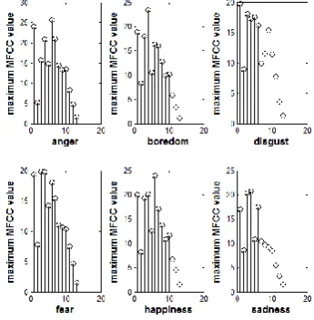
[image:2.595.53.277.263.389.2]where, S(p) is the log compression of the product of Mel-filter transfer function and the magnitude of the FFT. With M=33 in this work, the first 13 coefficients have been considered. Through experimentation it is observed that the emotion of anger (1st, 6th, 7th, 8th, 10th, 11th, 12th, 13th MFCC coefficients) followed by happiness (1st, 6th, 7th, 8th, 10th MFCC coefficients) exhibits the maximum values of MFCC across the 13 coefficients most of the times as seen in Fig. 3.
Fig 3: Trend of maximum value of MFCC across the 13 coefficients for various emotions
2.2.2 Pitch
The technique proposed by D. Talkin in [17] has been chosen to extract pitch. With pitch typically taking value as low as 60 Hz and as high as 400 Hz, the maximum value of pitch across each emotion is observed experimentally as shown in Table 1. The emotion of anger is observed to exhibit highest pitch while boredom emotion has the lowest pitch.
Table 1. Maximum values of pitch across each emotion
Emotion Maximum
pitch (Hz) Emotion
Maximum pitch (Hz) Anger 380.95 Happiness 372.14 Boredom 351.71 Sadness 355.92 Disgust 363.86 Neutral 372.80
Fear 365.88
2.2.3 Energy
Energy is extracted from a speech signal using Eq. (2),
( )2
1 F
E a b
b
(2) Here, F indicates the total number of samples in a frame, over which the energy of a given speech signal a is calculated. Observing energy over short-time window can help in making a decision as to whether the speech signal is voiced or unvoiced at a particular time [18]. The relevance of energy to emotion recognition can be observed through Fig. 4 in which the maximum value of energy across the speech samples of Pre-emphasis Framing Windowing
Magnitude value of FFT Mel filtering
Log compression DCT MFCC
values
values
f (Hz)
F
il
ter m
ag
n
it
u
d
e
[image:2.595.62.281.497.562.2]Emo-DB is plotted. The emotion of anger is observed to exhibit maximum energy while disgust exhibits the lowest maximum energy.
Fig 4: Maximum value of energy
2.2.4 Spectral flux
Abrupt changes in the spectrum is captured by calculating the spectral flux [19] in which power spectrum for one frame is compared against the power spectrum from the previous frame for a total number of A samples/frame given by Eq. (3).
1 [ ( ) 1( )]2 1
A
SF Xk b Xk b
k b
A
(3)
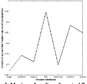
Xk(b) and Xk-1(b) are the spectral magnitudes of the current frame k and the previous frame k-1 respectively for a given number of frames per speech sample. The relevance of spectral flux to emotion recognition is observed in Fig. 5 where fear shows the highest maxima across the median values of spectral flux of all fear samples while the lowest value has been recorded for anger.
Fig 5: Maxima of median of spectral flux
2.2.5 Spectral roll-off
Spectral roll-off [20] is the frequency below which d % of the total energy falls, i.e. below what frequency is the d % of the magnitude distribution concentrated. It is given by Eq. (4). ( )2 ( )2
1 1
Roll off F
Ya q d Ya q
q q
(4) Here, F is the total number of samples in a given frame over
[image:3.595.96.239.422.561.2]which the concentrated magnitude distribution has been obtained, Ya(q) represents the qth frequency bin of the spectrum at frame a and d is usually 85% or 95%. The relevance of spectral roll-off to emotion recognition can be observed in Table 2. Among the maximum roll-off values across the archetypal emotions, fear records the highest while disgust records the lowest in the range of maximum values.
Table 2. Range of maximum roll-off values
Emotion
Maximum Roll-off
(Hz)
Emotion
Maximum Roll-off
(Hz) Anger 108.50 Happiness 107.04 Boredom 104.25 Sadness 91.66
Disgust 87.16 Neutral 110.76 Fear 129.67
2.2.6 Spectral stationarity
Spectral stationarity captures the fluctuations in the voice signal and is measured using Eq. (5),
0.2 [0,1] ( , 1) 0.8 SS
i itakura f fi i (5) Its significance is indicated by the fact that the spectral characteristics of adjacent frames are very similar if its value is close to one else the frames show high degree of difference [21]. Here, the function itakura () gives the itakura distortion measure between the current speech frame fi and the previous speech frame fi-1 [22]. The relevance of spectral stationarity to emotion recognition can be observed in Fig. 6.
Fig 6: Median of the mean of spectral stationarity
As can be observed, disgust shows the highest median value while fear shows the lowest. There exists a challenge for the feature classifier on receiving spectral stationarity values at its input as it is clearly evident from the fact that the median values recorded across all the emotions lies in the narrow range of 0.34 to 0.41. This will help in judging the accuracy with which the feature classifier works when encountered with such closely related feature values.
2.3
Dimensionality reduction
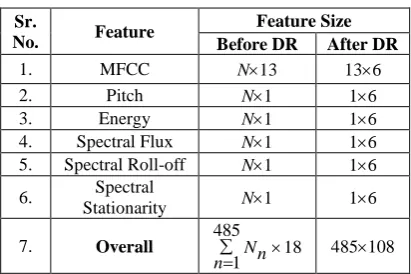
‘Curse of dimensionality’, a term coined by R. Bellman, occurs when the dimensionality of the input features is very large such that a higher requirement of volume of space is needed making the available data look very sparse. Adding to this problem is the fact that all the samples of Emo-DB are of different lengths and therefore the statistical method to dimensionality reduction has been adopted wherein mean, variance, median, maximum, minimum and index of dispersion across all frames have been calculated.
reduced to 485108 after dimensionality reduction irrespective of the number of frames.
Table 3. Impact of Dimensionality Reduction (DR)
Sr.
No. Feature
Feature Size Before DR After DR
1. MFCC N13 136
2. Pitch N1 16
3. Energy N1 16
4. Spectral Flux N1 16
5. Spectral Roll-off N1 16 6. Spectral
Stationarity N1 16
7. Overall 485 18 1Nn
n 485108
2.4
Feature Classification [23, 24, 25]
SVM differs from other approaches (like HMM, GMM, etc.) in the sense that it is a discriminant based method and does not estimate the probability of a given feature xto be lying in a given emotional class Ci for an emotion with label i, but is concerned in learning the discriminant (or the boundary) that separates emotions of one class from the other. This discriminant function is a linear combination of the components of the feature x and is expressed as,g x( ) w x b (6) where, w is a weight vector and b is termed as a bias or threshold weight. The equation g(x) = 0 is the decision surface called the ‘hyperplane’ that separates the extracted features of one class from other. The main intention of a discriminant method is to not only place the features on the correct side of the hyperplane but also to keep them some distance away, for which it is the discriminant function g(x) that gives an algebraic measure of the distance from feature x to the hyperplane. Given a two class problem, if the features of one class are labeled by r = +1 and the features of the other class are labeled by r = -1, then the combined discriminant function becomes as shown in Eq. (7).
(r w x b) 1 (7) The term ‘support vectors’ play an important role in SVM and are obtained by considering the equality in Eq. (7) to hold true such that only those features lying along the margin (close to the boundary) will be considered.
2.4.1 Optimization
To train the SVM, one begins with a standard optimization problem that involves minimizing w2 2 subject to the constraints of Eq. (7). This is equivalent to maximizing the margin for which w2is minimized. In a situation where the training data is not linearly separable, the task is equivalent to looking for a hyperplane that will incur the least error (if any). A slack variable i 0 is defined that stores the deviation from the margin such that it caters to either a feature lying on the wrong side of the hyperplane or lying on the right side but within the margin (such that it is not sufficiently away from the hyperplane). To assign an extra cost for an incurred error, the earlier objective function is modified to w2 2 C i
i
where C is the penalty (regularization) factor that penalizes not only the misclassified points but also the ones within the margin for better generalization. The significance of C parameter is that small C implies a small penalty thereby
indicating a large margin while a large C implies a large penalty indicating a narrow margin.
2.4.2 Kernelization
Kernel function involves mapping the input vectors into high-dimensional feature vector space after which the training data can be linearly separated such that the SVM which lives in the high-dimensional space roughly takes the same amount of time for training as it would take on an unmapped data (in the original feature space). Different kernels explored in the research towards SER include the following:
(i) Linear: K(xi,xj) = xiTxj (8) (ii) Polynomial: K(xi,xj) = ( )
T d
xi xj r
, 0 (9)
(iii) Radial basis: K(xi,xj) =
2
exp( xixj ), 0 (10) (iv) Sigmoid: K(xi,xj) = tanh( xiTxj+r), 0 (11)
2.4.3 Grid Search
The ultimate goal of SVM which involves feature classification (in our case recognizing the emotion in an unknown test sample), will only be possible by identifying the optimum value of (C, ). C caters to the trade-off between the margin size and the amount of error occurred thereby and forms an integral parameter of the kernel function. To determine their optimal values, the concept of ‘grid search’ finds usefulness in which various pairs of (C, ) are tried and the one with best prediction accuracy is selected. This search can be fine-tuned and made less time consuming by first identifying the range of (C, ) over which an appreciable accuracy could be achieved following which, conducting a finer grid search along the neighborhoods of this chosen range, the desired value of (C, ) can be obtained in a relatively shorter time.
2.4.4 Cross-validation
Estimating how accurately a trained model will perform when encountered with unknown test samples that belong to the same population and thereby generalizing to any independent data set is the basis of cross-validation (CV). Owing to the limitedness of a given data set, cross-validation involves partitioning the entire dataset into complimentary subsets such that the learning process is carried out using one subset (called the training set) and the validation of the learning is carried out on the complimentary subset (called the validation set). To estimate the expected level of fitness of a trained model to a dataset that is independent of the data that were used to train the model, a third set i.e. a testing set comprising of data samples ‘held out’ from training is considered. Thus, a given feature dataset is split into not two but three independent subsets viz. training set, validation set and testing set. The non-exhaustive cross-validation technique of k-fold CV has been chosen in which the original dataset is randomly partitioned into k equal size subsets. A single subset is then retained as the validation set for testing the model that has been fit on the training set formed from the remaining (k-1) subsets. The cross-validation is then repeated k times, with each of the k subsets used exactly once as the validation data.
2.4.5 Multi-class SVM
class that will be labeled as +1 and the remaining feature vectors (from other classes) that will be labeled as -1. As in the classic case of ‘winner takes all’, the strategy thus becomes choosing that class corresponding to the unknown test sample which will give the maximum value of the discriminant function assigned to it.
3.
EXPERIMENTAL SETUP
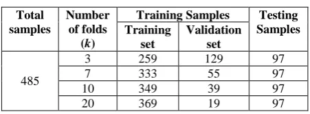
[image:5.595.54.280.337.420.2]Using Emo-DB, the parametric representations of speech in the form of MFCC, energy, pitch, spectral roll-off, spectral stationarity and spectral flux have been extracted. From each emotional class, 80% have been used for training (and validation) the chosen classifier of SVM and the remaining 20% have been used for testing the performance of the trained SVM. It has been observed that larger the number of folds, smaller is the bias of the estimator and therefore accurate will be the results. Keeping this in mind, experimentations have been carried out by increasing the number of folds and seeing its effect on the overall classification accuracy. Thus, the values of k have been taken as 3, 7, 10 and 20 respectively and thereby, the number of samples that have been used for training and testing are mentioned in Table 4.
Table 4. Number of samples from Emo-DB used for training and testing
Total samples
Number of folds
(k)
Training Samples Testing Samples Training
set
Validation set
485
3 259 129 97
7 333 55 97
10 349 39 97
20 369 19 97
The choice of one-v/s-all SVM with linear, polynomial and radial basis function (RBF) kernels has been made. The performance of the SVM as a classifier of emotions has been scrutinized by observing for which of the chosen features is the average classification accuracy the maximum. Based on the confusion matrix obtained for the best chosen features, corresponding precision, recall and F-score values have also been obtained. For the task of emotion recognition, precision is the fraction of correctly recognized emotion speech instances (across a given emotion) that are relevant to the result while recall is the fraction of the emotion speech instances that are relevant to the query successfully retrieved. Taking twice the harmonic mean of the calculated precision and recall values is the metric of F-score.
Along with multi-class SVM, a binary classification has also been experimented wherein classification into positive v/s negative valence, positive v/s negative arousal and neutral v/s emotion has been conducted across the archetypal emotions whose bifurcation is as seen from Table 5.
Table 5. Valence and Arousal emotion sets
Valence Arousal Positive Negative Positive Negative Happiness Anger Anger Boredom Sadness Boredom Disgust
Disgust Fear Fear Happiness Sadness
4.
RESULTS
The % accuracy for the chosen features of MFCC, energy, pitch, spectral roll-off, spectral stationarity and spectral flux is as shown in Table 6.
Table 6. Accuracy of the chosen features
Sr.
No. Features
Type of kernel
No. of
folds (k) Accuracy
1. MFCC Poly. 3 77.32%
2. Pitch RBF 20 49.48%
3. Spectral
roll-off linear 10 47.42% 4. Spectral
stationarity RBF 7 42.27% 5. Spectral
flux linear 3 37.11%
6. Energy RBF 3 31%
It is observed that the best emotion recognition rate is achieved through MFCC. The accuracy obtained from other features by considering them individually is very low in comparison to that of MFCC. Thus, the best way in improving the overall accuracy of the SER system is by finding out which of the remaining five features could suitably be appended to MFCC frame-wise. Through experimentation, it has been found out that the choice of MFCC, energy, pitch, spectral roll-off, spectral stationarity and spectral flux together has yielded the best average accuracy of 86.6% using the RBF kernel and cross-validation with k=20. The corresponding confusion matrix for this set of features is shown in Table 7.
Table 7. Confusion matrix
(Emotions (EM) - A: Anger, B: Boredom, D: Disgust, F: Fear, H: Happiness, S: Sadness, N: Neutral)
EM A B D F H S N
A 100 0 0 0 0 0 0 B 0 100 0 0 0 0 0
D 0 0 25 62.5 0 12.5 0
F 8.33 0 0 58.34 33.33 0 0
H 7.69 0 0 0 92.31 0 0
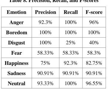
S 0 0 0 0 0 90.91 9.09 N 0 0 0 0 0 0 100 As seen from the confusion matrix in Table 7, the emotion of disgust after testing got wrongly misclassified with fear and sadness respectively. Similarly, the emotion of fear got confused with happiness and anger respectively. Based on the confusion matrix, the precision, recall and F-score is shown in Table 8. The significance of higher precision implies more relevant results being returned while higher recall implies returning most of the relevant results only. As can be viewed from Table 8, the precision, recall and F-score values are showing comparatively smaller values for disgust and fear respectively.
Table 8. Precision, Recall, and F-scores
Emotion Precision Recall F-score
Anger 92.3% 100% 96% Boredom 100% 100% 100%
Disgust 100% 25% 40% Fear 58.33% 58.33% 58.3% Happiness 75% 92.3% 82.75%
Sadness 90.91% 90.91% 90.91% Neutral 93.33% 100% 96.55%
Table 9. % Accuracy across binary and multi-class SVM
Type of
classification Features Kernel Folds Accuracy +ve v/s –ve
Arousal 1. MFCC 2. Pitch 3. Energy 4. SF 5. SR 6. SS
Poly. 3 100%
Neutral v/s
Emotion RBF 20 97.94%
+ve v/s –ve
Valence Poly. 20 96.38% Multi-class RBF 20 86.6%
5.
CONCLUSION
In this work, creating an SER system that chooses features relevant to the recognition of emotions has been aimed. With the choice of MFCC, energy, pitch, spectral flux, spectral roll-off and spectral stationarity, emotion recognition through the speech samples of Emo-DB has been performed by training and testing the feature classifier of SVM. An average accuracy of 86.6% has been obtained by considering the six chosen features as input to the SVM. This accuracy has further increased to 100% by considering the binary form of SVM that classifies the chosen emotions into positive v/s negative arousal thereby indicating the fact that as the number of classes increase, the accuracy with which the SVM classifier will perform is bound to decrease.
6.
REFERENCES
[1] Rong, J., Li, G and Chen, Y. Acoustic feature selection for automatic emotion recognition from speech. Information Processing and Management. (May 2009), 315-328.
[2] Batliner, A. et al. The automatic recognition of emotions in speech. Emotion-Oriented Systems. 2011, 71-99. [3] Davis, S. and Mermelstein, P. Comparison of parametric
representations for monosyllabic word recognition in continuously spoken sentences. IEEE Trans. on Acoustics, Speech and Signal processing. (Aug. 1980), 357-366,
[4] Chapaneri, S. Spoken Digits Recognition using Weighted MFCC and Improved Features for Dynamic Time Warping. Intl. Journal of Computer Applications. (Feb.2012), 6-12.
[5] Pao, T., Chen, Y., Yeh, J. and Liao, W. Detecting emotions in Mandarin speech. Computational Linguistics and Chinese Processing. (Sep 2005), 347-361.
[6] Kumar, K., Kim, C. and Stern, R. Delta-spectral Cepstral Co-efficients for robust speech recognition. IEEE Intl.
Conf on Acoustics, Speech and Signal Processing. (May 2011), 4784-4787.
[7] Zhou, G., Hansen, J. and Kaiser, J. Nonlinear feature based classification of speech under stress. IEEE Trans. on Speech and Audio Processing. (Mar. 2001), 201-216. [8] Lee, C. and Narayanan, S. Towards detecting emotions
in spoken dialogs. IEEE Trans. on Speech and Audio Processing. (Mar. 2005), 293-303.
[9] Wu, S., Falk, T. and Chan, W. Automatic speech emotion recognition using modulation spectral features. Speech Communication. (Sep. 2010), 768-785.
[10]Fewzee, P. and Karray, F. Dimensionality reduction for emotional speech recognition. IEEE Intl. Conf. on Social Computing and Intl. Conf. on Privacy, Security Risk and Trust. (Sep. 2012), 532-537.
[11]Zou, H. and Hastie, T. Regularization and variable selection via the elastic net. Journal of the Royal Statistical Society. (Apr. 2005), 301-320.
[12]Yu, L. and Liu, H. Feature selection for high-dimensional data: a fast correlation-based filter solution. Proceedings of the 12th Intl. Conf. on Machine Learning. 2003, 856-863.
[13]Albornoz, E., Milone, D. and Rufiner, H. Spoken emotion recognition using hierarchical classifiers. Computer Speech & Language. (Jul. 2011), 556-570. [14]Seehapoch, T. and S. Wongthanavasu. Speech emotion
recognition using Support Vector Machines. 5th IEEE Intl. Conference on Knowledge and Smart Technology (KST). (Jan. 2013), 86-91.
[15]Burkhardt, F. et al. A database of German emotional speech. INTERSPEECH. 2005, 1-4.
[16]Combrinck, H. and Botha, E. On the mel-scaled cepstrum. University of Pretoria. 1996.
[17]Talkin, D. A robust algorithm for pitch tracking. Speech Coding and Synthesis. 1995, 495-518.
[18]Rabiner, L. and Schafer, R. Introduction to digital speech processing. Foundations and trends in signal processing. (Jan. 2007), 1-194.
[19]Polzehl, T., Schmitt, A., Metze, F. and Wagner, M. Anger recognition in speech using acoustic and linguistic cues. Speech Communication. (Jan. 2013), 1-14. [20]Eyben, F., Wollmer, M. and Schuller, B.
OpenEAR-introducing the Munich open-source emotion and affect recognition toolkit. 3rd Intl. Conf. on Affective Computing and Intelligent Interaction and Workshops. (Sep. 2009), 1-6.
[21]Finkelstein, S. et al. Investigating the influence of virtual peers as dialect models on students’ prosodic inventory. INTERSPEECH. (Sep. 2012), 60-67.
[22] Buzo, A., Gray, A., Gray, R and Markel, J. Speech coding based upon vector quantization. IEEE Trans. on Acoustics, Speech and Signal processing. (Oct. 1980), 562-574.
[23]Alpaydin, E. Introduction to machine learning. ISBN-978-81-203-4160-9. 2012.
[24]Burges, C. A tutorial on Support Vector Machines for pattern recognition. Data Mining and Knowledge Discovery. (Jun. 1998), 121-167.
[image:6.595.50.288.253.375.2]