Some Improvement on Convergence Rates of Kernel Density Estimator

(1)

http://dx.doi.org/10.4236/am.2014.511161

Some Improvement on Convergence Rates

of Kernel Density Estimator

Xiaoran Xie, Jingjing Wu

Department of Mathematics and Statistics, University of Calgary, Calgary, Canada Email: [email protected], [email protected]

This work is licensed under the Creative Commons Attribution International License (CC BY). http://creativecommons.org/licenses/by/4.0/

Abstract

In this paper two kernel density estimators are introduced and investigated. In order to reduce bias, we intuitively subtract an estimated bias term from ordinary kernel density estimator. The second proposed density estimator is a geometric extrapolation of the first bias reduced estimator. Theoretical properties such as bias, variance and mean squared error are investigated for both estimators. To observe their finite sample performance, a Monte Carlo simulation study based on small to moderately large samples is presented.

Keywords

Kernel Density Estimation, Geometric Extrapolation, Bias Reduction, Mean Squared Error, Convergence Rate

1. Introduction

Many efforts have been devoted to investigating the optimal performance of kernel density estimator since it has been the most widely used nonparametric method in the last decades. Suppose we use fn

( )

x to denote the

kernel estimator of the true density function f x

( )

. Normally we use mean squared error (MSE) and its two components, namely bias and variance, to quantify the accuracy of an estimator. Note that the MSE of fn

( )

x

is decomposed into two parts:

( )

(

)

(

( )

)

(

( )

)

(

( )

)

( )

(

)

(

( )

)

2 2 2

2

MSE

Bias Var .

n n n n n

n n

f x E f x f x Ef x f x E f x Ef x

f x f x

= − = − + −

= +

(2)

asymptotic convergence rate

2 2 1

r r O n_ − + _

  of MSE for orthogonal kernel estimators. Article [2] introduced geo-

metric extrapolation of nonnegative kernels, while [3] discussed the number of vanishing moments of kernel or-der using Fourier transformation. Variable kernel estimation in [4] successfully reduced the bias by employing larger smoothing parameters in low density regions, while [5] introduced the idea of inadmissible kernels which also results in reduced bias. On the other hand, [6] proposed an estimator using some probabilistic arguments which achieves the goal of bias reduction. Article [7] suggested a locally parametric density estimator, a semi-parametric technique, which effectively reduces the order of bias. Article [8] proposed algorithms relevant to quadratic polynomial and β cumulative distribution function (c.d.f.) which accommodates possible poles at boundaries and in consequence reduces the bias at boundaries. Article [9] introduced a bias reduction method using estimated c.d.f. via smoothed kernel transformations. Article [10] introduced a two-stage multiplicative bias corrected estimator. Article [11] developed a skewing method to reduce the bias while the variance is only increased by a moderate constant factor. In addition, some recent works discussed approaches of obtaining smaller bias of the estimator via several other methods. Article [12] worked out a bias reduced kernel relative to the classical kernel estimator via Lipschitz condition. Article [13] introduced an adjusted kernel density estima-tor in which the kernel is adapted to the data but not fixed. This method naturally leads to an adaptive-choice of the smoothing parameters which can reduce the bias.

Although the variance reduction method is not as approachable as the bias reduction method, there still have been a lot of scholars working on it. Article [14] suggested an approach to reduce the variance in local linear re-gression employing the idea of the skewing method. Article [15] also used the skewing method on bias reduc-tion and variance reducreduc-tion at the same time which in turn reduces the MSE.

Many of above mentioned bias reduction methods result in complex kernel density estimators. In this paper, we introduce a novel but intuitive and feasible bias reduced kernel density estimator. In Section 2, we present the bias reduced estimator and investigate its asymptotic bias, variance and MSE. A second estimator is pro-posed and studied in Section 3 as a geometric extrapolation of the bias reduced kernel. To examine the finite sample performance of both estimators, a simulation study is carried out in Section 4. Finally some remarks are given in Section 5.

2. A Bias Reduced Kernel Estimator

Kernel density estimator was first introduced in [16] and [17]. Suppose X1,,Xn is a simple random sample

from the unknown density function f. Let K be a function on real line, i.e. the “kernel”, and let h be a positive value, i.e. the “bandwidth”. Then the kernel density estimator of f is defined as

( )

1

.

n

i n

i

x X

f x K

nh = h

−   = _ _  

∑

(2.1) To make the estimator meaningful, the kernel function is usually required to satisfy conditions K x

( )

>0,

( )

d 1

K x x=

∫

and

∫

_{x K}2

( )

_x _d_x_{< ∞}

. Both [18] and [19] pointed out that if

∫

uK u

( )

du=0 and f is twice con-tinuously differentiable in a neighborhood of x, then

( )

(

)

(

( )

)

( )

1

( )

2 2

( )

3

Bias d

2

n n

f x =E f x −f x = f′′ x h

∫

u K u u+O h (2.2) and

( )

(

)

1

( )

2

( )

(

( )

1

)

Var fn x f x K u du o nh .

nh

−

=

_∫

+ (2.3)

Then from (2.2) and (2.3) we have

( )

(

)

(

( )

)

(

( )

)

( )

(

)

( )

2

2 ₄ ₂ ₂

MSE Bias Var

1 1

d d .

4

n x n x n x

x

f f f

f h u K u u f K u u

nh x

= +

 

′′ _

_∫

_ +

_∫



We can easily see that the optimized bandwidth is

1 5

h O n__ − __

 

(3)

4 5

n− .

In order to reduce the bias of ordinary kernel density estimator, we can intuitively subtract the leading bias term 1

( )

2 2

( )

d

2f′′ x h

∫

u K u u in (2.2) from it. Since the leading term of the bias is unavailable due to the

unknown f, we can simply use its estimation, i.e.

( )

_Bias

₍

_{( )}

₎

_.

n x n x n x

f = f − f



One could use any type of estimation of the bias term. We could simply replace f with the kernel estimator fn

since it is readily available. As a result, our proposed estimator is

( )

2

( )

2

( )

2

( )

1 1

1

d d .

2 2

n n

i i

n n n

i i

x X x X

h h

f x f x f x u K u u K u K u u K

nh = h n = h

− −     ′′ ′′ = − = _ _− _ _    

∑

∫

 _(2.4)

From the way of construction, this new estimator should be able to reduce the bias and thus the MSE. To see whether this is the case or not, we next calculate the bias and the variance of fn

( )

x . We make the following

regularity condition on f, K and h: 1)

∫

uK u

( )

du=0.

2) f is fourth differentiable in a neighbourhood of x. 3) h→0 and nh→ ∞ as n→ ∞.

Theorem 2.1. Under 1), 2) and 3),

( )

(

)

3

( )

3

( )

4

Bias d

6

n

h

f x = − f′′′ x

∫

u K u u+O h (2.5) and

( )

(

)

( )

(

( )

)

2

( ) ( )

₂

( )

2 1

1

Var d d .

2

n

f x f x u K u u K u u O n

nh

− ′′

=

_∫

+

 _(2.6)

Consequently,

( )

(

)

(

6

( )

1

)

MSE fn x O h nh −

= +



and the optimal MSE is of the order

6 7

O n_ − _

  with

1 7

h= O h_ − _

 .

Proof. By Taylor expansion we have

( )

(

)

( )

( ) (

)

( ) ( )

( )

2 3 4

2 3

2 3 4

1

d d

1 1

d

2 6

d d ,

2 6

n

x t

E f K f t t K u f x hu u

h h

K u f x huf x hu f x hu f x u O h

h h

f x f x u K u u f x u K u u O h

x = _ − _ = −

   _′ _′′ _′′′  = _ − + − _ +   ′′ ′′′ = + − +

∫

( )

(

)

( )

( ) (

)

( )

3 3 1 2 2 2 2 2 1 1 d 1 d d 1 d 2 d . 2 n i n i

x X x t

E f x E K K f t t

h h

nh h

x t

K f t t K u f x hu u

h h

K u f x huf x hu f x u o h

h

f x f x u K u u o h

(4)

Thus we have

( )

(

)

(

( )

)

( )

(

)

( )

(

( )

)

( )

(

( )

)

( )

2 2

3 4 ₂

3 4 2 4

3 3 4 Bias d 2 d d 6 4 d . 6 n n n n

f x E f x f x

h

E f x f x E f x u K u u

h h

f x u K u u O h f x u K u u o h

h

f x u K u l u O h

= − ′′ = − − ′′′ ′′′′ = − + − + ′′′ = − +

∫

  (2.8)

On the other hand,

( )

(

)

( )

(

)

( )

(

)

(

( )

)

(

( )

)

2 2 2 2 4 2 2

Var Var d

2

2Var 2Var d

2

2Var d Var .

2

n n n

n n

h

f x f x f x u K u u

h x

x

f f x u K u u

h

f u K u u f x

  ′′ = _ − _    _′′  ≤ + _ _   ′′ = +

∫

 (2.9)

Note that (2.7) gives

( )

(

)

( )

( ) ( ) (

)

(

( )

)

( ) ( ) ( )

(

( )

)

( ) ( )

1 3 6 1 2 2 6 6 2 2 2 5 2

2 2 2

5

1 1

Var Var Var

1 1 d d 1 1 d 1 1 d 1 n i n i

x X x X

f x K K

h h

nh nh

x t x t

K f t t K f t t

h h

nh nh

K u f x hu u f x O h

n nh

h

K u f x huf x O h u f x O

n n nh n =   −    −  ′′ = _ ′′_ __= _ ′′_ __         −  −      ′′ ′′ = _ _ − _ _ _ _       ′′ ′′ = − − +   ′′ ′ ′′ = − + − _{+  }   =

∑

∫

( ) ( ) ( )

₂

(

( )

1

)

4

5 f x K u du O nh .

h

−

′′ +

∫

(2.10)

Finally (2.9) and (2.10) together with (2.3) gives (2.6). 

Remark 2.1. From Theorem 2.1 we can see that if K is symmetric, i.e. K u

( )

=K

( )

−u , then all the odd mo-ments of K are zero and, as a result, the bias of fn

( )

x will be improved to a higher order of

( )

4

O h . In this case, the optimal MSE is further reduced to

8 9

O n_ − _

  with

1 9

h= O n_ − _

 .

Remark 2.2. From the definition of fn in (2.4), this estimator could be possibly negative on some points x.

In order to make it meaningful in practice, i.e. make it a positive density estimator, one can use the following variation of the proposed bias deducted estimator

( )

( ( ) )

( )

₍ _{( )} ₎ 0 0 ˆ _, d n n

n _f _x

n

n f x

f x I f x

f x I x

> > =

∫

   

where IA is an indicator function that takes value one on set A and zero otherwise. Note that the first term on

the right hand side of Equation (2.4) converges to f x

( )

in probability, while the second term is of the order

( )

O h , which goes to zero as n→ ∞ under 3). Thus fn

( )

x converges to f x

( )

in probability, and as a re-

sult fn

( )

x is positive in probabililty at any point x∈Ω with Ω the support of f. Therefore, ˆfn has similar

(5)

3. A Geometric Extrapolated Kernel Estimator with Bias Reduction

Geometric extrapolation was introduced in kernel density estimation by [2]. Consider the ordinary kernel density estimator with two different bandwidths h and 2h:

( )

1 1 , n i h i x X

f x K

nh = h

−   = _ _  

∑

( )

2 1 1 . 2 2 n i h i x X

f x K

nh = h

−

 

= _ _

 

∑

Suppose the kernel function K above is symmetric so that all the odd moments of K are zero. Article [2] pro-posed the following estimator

( )

43

( )

13

( )

2 4 1 3 3 1 1 1 1 . 2 2

n h h

n n

i i

f x f x f x

x x x x

K K

nh h nh h

− − = = =   −    −  =_ _ __ ×_ _ __     

∑

 

∑

  (3.1)

Note that fn

( )

x



doesn’t have integral one. In order to improve the MSE of order

4 5

O n_ − _

  of the ordinary

kernel estimator, one has to relax the constraint of integrating to one. The powers 4 3 and

1 3

− are selected to reduce the bias of the ordinary kernel estimator to _{O h}

( )

4

. Consequently, the MSE of fn

( )

x



is improved to the order of

8 9

O n_ − _

 , which is a faster convergence rate than the rate

4 5

O n_ − _

  of the ordinary kernel

estima-tor.

Instead of using the ordinary kernel estimator, we propose to use the bias reduced kernel estimator, presented in Section 2, in the construction of geometric extrapolated kernel (3.1). Denote the bias reduced kernel estimator with two bandwidths h and 2h as

( )

2 2

( )

1 1 1 d , 2 n i h h i x x

f x K f x h u K u u

nh = h

−   _′′ = _ _−  

∑

∫



( )

2 2

( )

2 2

1

1 1

d .

2 2 4

n

i

h h

i

x x

f x K f x h u K u u

nh = h

−   _′′ = _ _−  

∑

∫



Now the geometric extrapolated kernel estimator with bias reduction is proposed as

( )

87

( )

17

( )

2 .

n h h

f x = f x f− x

  

(3.2) Since the bias reduced kernel estimator has improved bias and MSE over the ordinary kernel estimator, espe-cially when K is symmetric, we expect that with geometric extrapolation it will achieve further improvement.

Theorem 3.1. Under 1), 2) and 3),

( )

(

)

(

( )

)

2

( )

(

( )

₁

)

2 4 4 5

2 1

Bias d d

7 21

n

f x =_ u K u u − u K u u f_ ′′′′ x h +O h + nh −



∫







and

( )

(

)

( )

(

1 2

( )

2

)

2

8 1

Var Var .

7 7

n h h

f x = _ f x − f x _+O n h− + nh −

 



  

Consequently,

( )

(

)

(

8

( )

1

)

MSE fn x O h nh −

= +



(6)

and the optimal MSE is of the order

8 9

O n_ − _

  with

1 9

h= O h_ − _

 .

Proof. We calculate Bias

(

f_h

( )

x

)

first. Similar argument to (2.8) gives

( )

(

)

(

( )

)

( )

( ) ( )

( )

(

( )

)

2 2 4 2 3 ₂

3 4 4 2

d 2

1 1 1

d d d .

6 4! 2 2!

h n n

h

E f x E f x E f x u K u u

h

f x f x u K u u h f x u K u u u K u u

′′ = − _ _  ₋ ₋  ′′′ ′′′′ = − +  − +    

∫

 

Let Jh

( )

x =Efh

( )

x , then

( )

₁

_{( )}

3 3

_{( )}

4 4 _,

h

b b

J x f x h h

f x f x

 

= _ + + + _

 

  (3.3)

where

( )

2

₍

( )

₎

2

( )

2

( )

1 d , 3

!

1 d 1 d d , 4, 5, .

! 2 2 !

i

i i

i i i

i i i i

f x

u K u u i

i b

f x f x

u K u u u K u u u K u u i

i i − −  − =   =   − − − ⋅ =  ₋ 

∫



Taking logarithm of (3.3) gives

( )

(

)

(

( )

)

_{( )}

( )

(

)

( )

_{( )}

3 4 3 4 1 3 4 3 4 1

log log log 1

1 log ! h i i i b b

J x f x h h

f x f x

b b

f x h h

i f x f x

− ∞ =   = +  + + +        − = +  + +     

∑

  (3.4)

Here we want to construct a geometric extrapolated kernel estimator of the form 1

( ) ( )

2 2

t t

h h

f x f x

  _{that possibly}

reduces the bias. In another word, we need t₁log

(

J_h

( )

x

)

+t₂log

(

J₂_h

( )

x

)

has term log

(

f x

( )

)

but has 3

h

term disappear. Thus t1 and t2 have to satisfy

1 2 3 1 2 1 2 0. t t t t + =   + = 

The solution to above equation system is 1

8 7

t = and 2

1 7

t = − , and this gives our proposed estimator (3.2). Now

( )

(

)

(

( )

)

(

( )

)

_{( )}

4 4

( )

5 2

8

8 1

log log log

7 h 7 h 7

b

J x J x f x h O h

f x

− = − +

and a series expansion for exponential function gives

( )

8 1 4 5 7 7 2 4 8 . 7 h h

J x J− x = f x − b h +O h (3.5) We rewrite

( )

,

h h

f x =J x +U 

( )

2h 2h ,

f x =J x +V 

(7)

( )

_{( )}

( )

_{( )}

( )

_{( )}

( )

_{( )}

( )

_{( )}

( )

_{( )}

8 1

8 1 8 7 1 7

7 7 7 7

2 2 2 2 2 8 1 7 7 2 2 2 1

8 1 7

7 7 2 2 2 1 1 8 1 1 1 7 7 8 1 7 7

h h h h

h h

h h h h

h h

U V

f x f x J x J x

J x J x

U U V V

J x O J x O

J x J x J x J x

J x J x

J x J x U V

J x J x

− − − − −     = _ + _ _ + _          _ _   _ _        = _ + + __ _ __⋅ _ − + __ _ __               = + _ _ −    

(

)

(

)

8 7 2 ,

O U V

  + +       and then

( )

(

)

( )

(

( )

)

( )

(

)

8 1 7 7 2 1 4 5 4 1 4 5 4 Bias 8 0 0 7 8 . 7

n h h

f x E f x f x f x

b h O h O nh

b h O h nh

− − −   = _ _−   = − + + + + = − + +   

Since

( )

3

2 1 h h J x O h

J x = + by (3.4), the variance of fn

( )

x  is

( )

_{( )}

( )

_{( )}

(

)

( )

(

( )

)

(

( )

)

( )

(

( )

)

( )

(

)

1 8

8 1 ₇ ₇

2 7 7 2 2 2 2 3 2 2 1 2 2 1 8 1 Var Var 7 7 8 1 Var 1 7 7 8 1 Var 7 7 . h h h h h h h h h h

J x J x

f x f x U V O U V

J x J x

f x f x O h O nh

f x f x O n h nh

O nh − − − − −         _ _ =   −   + +   _ _         _     _     = _ − _ + +     = _ − _+ +   =        Remark 3.1. Article [2] proposed the geometric extrapolation of ordinary kernel estimator which results in optimal MSE of the order

8 9

O n_ − _

 . Though here we achieve the same order of optimal MSE, we don’t impose

the assumption that K is symmetric while [2] does.

Remark 3.2. When K is symmetric, we propose another estimator

( )

16

( )

1

15 15

2 .

n h h

f x = f x f x −

  

This estimator reduces the bias to

( )

6

O h and has improved optimal MSE of the order

12 13

O n_ − _

  with

1 13

h= O n_ − _

 .

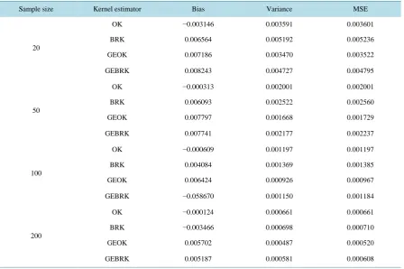
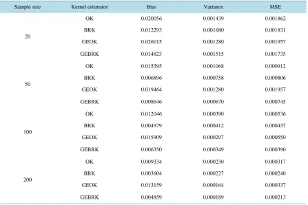
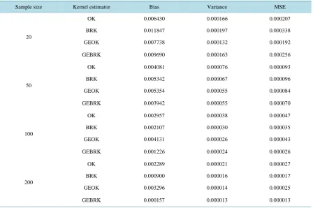
4. Simulation Study

(8)

bias reduced kernel estimator (GEBRK) fn



given in (3.2). Particularly, we compare their bias and MSE with the ordinary kernel density estimator (OK) fn in (2.1) and the geometric extrapolation of ordinary kernel

esti-mator (GEOK) fn



in (3.1).

Without loss of generality, we suppose f is the standard normal density. We randomly select 1000 indepen-dent samples of size n = 20, 50, 100 or 200. We choose arbitrarily the points x = 0, 0.5, 1, 1.5, 2, 2.5 and 3 at which the kernel estimators are calculated and compared. Since the properties of kernel estimators do not de-pend much on which particular kernel is used, we choose the standard normal as the kernel function K without loss of generality. For the bandwidth h, we use the optimal one for each individual kernel estimator. In another word, since here K is symmetric, by Remarks 2.1 and 3.2, we choose h=n−1 5 for OK, h=n−1 9 for both BRK and GEOK and h=n−1 13 for GEBRK. The bias, variance and MSE are estimated respectively by

( )

1000

(

)

0 1

1

ˆ ˆ

Bias ,

1000i i

θ θ θ

=

∑

−

( )

1000

( )

2 1000

1 1

ˆ ˆ ˆ ˆ ˆ

Var with

1000 i i 1000i i

θ θ θ θ θ

= =

=

∑

− =

∑

and

( )

1000

(

)

₂

0 1

1

ˆ ˆ

MSE ,

1000 i i

θ θ θ

=

∑

−

where θ0 is the true parameter and ˆθi is the estimate value ˆθ based on the i-th sample. In our case, θ =0

( )

f x and ˆθ is either fn

( )

x , fn

( )

x



, fn

( )

x or fn

( )

x



for fixed x = 0, 0.5, 1, 1.5, 2, 2.5 or 3. The simulation results are presented inTables 1-7.

FromTables 1-7 we can see that BRK consistently has smaller bias and MSE than OK except for x = 1. This is simply due to the fact that f′′

( )

1 =0 which in turn reduces the bias of OK to O h

( )

4 . Apparently this is of the same order as the bias of BRK, however this is a special case that is only true at point x = 1 here and the

Table 1.Bias, variance and MSE of different kernel density estimators evaluated at x = 0.

Sample size Kernel estimator Bias Variance MSE

20

OK −0.051923 0.003405 0.006101

BRK −0.028022 0.003849 0.004644

GEOK −0.036122 0.003106 0.004411

GEBRK −0.027881 0.003158 0.003935

50

OK −0.036192 0.002127 0.003437

BRK −0.017092 0.002105 0.002397

GEOK −0.025861 0.001686 0.002355

GEBRK −0.018000 0.001620 0.001944

100

OK −0.028514 0.001245 0.002058

BRK −0.012703 0.001132 0.001294

GEOK −0.021273 0.000885 0.001338

GEBRK −0.014114 0.000829 0.001028

200

OK −0.022334 0.000815 0.001314

BRK −0.009988 0.000691 0.000791

GEOK −0.017786 0.000531 0.000847

(9)

[image:9.595.86.541.99.397.2]

Table 2. Bias, variance and MSE of different kernel density estimators evaluated at x = 0.5.

20

OK −0.035504 0.003537 0.004798

BRK −0.015563 0.004579 0.004821

GEOK −0.021755 0.003326 0.003800

GEBRK −0.015037 0.003978 0.004204

50

OK −0.022483 0.002055 0.002560

BRK −0.007345 0.002321 0.002375

GEOK −0.013747 0.001689 0.001878

GEBRK −0.007874 0.001904 0.001966

100

OK −0.017031 0.001308 0.001598

BRK −0.005084 0.001334 0.001360

GEOK −0.011120 0.000978 0.001102

GEBRK −0.006062 0.001048 0.001085

200

OK −0.013480 0.000816 0.000998

BRK −0.003789 0.000793 0.000807

GEOK −0.009041 0.000569 0.000650

GEBRK −0.004779 0.000605 0.000628

Table 3. Bias, variance and MSE of different kernel density estimators evaluated at x = 1.

20

OK −0.003146 0.003591 0.003601

BRK 0.006564 0.005192 0.005236

GEOK 0.007186 0.003470 0.003522

GEBRK 0.008243 0.004727 0.004795

50

OK −0.000313 0.002001 0.002001

BRK 0.006093 0.002522 0.002560

GEOK 0.007797 0.001668 0.001729

GEBRK 0.007741 0.002177 0.002237

100

OK −0.000609 0.001197 0.001197

BRK 0.004084 0.001369 0.001385

GEOK 0.006424 0.000926 0.000967

GEBRK −0.058670 0.001150 0.001184

200

OK −0.000124 0.000661 0.000661

BRK −0.003466 0.000698 0.000710

GEOK 0.005702 0.000487 0.000520

[image:9.595.93.542.424.722.2]

(10)

[image:10.595.87.539.99.397.2]

20

OK 0.019396 0.002676 0.003052

BRK 0.017134 0.003727 0.004021

GEOK 0.025892 0.002580 0.003250

GEBRK 0.019406 0.003468 0.003845

50

OK 0.013847 0.001334 0.001525

BRK 0.010788 0.001646 0.001763

GEOK 0.020440 0.001163 0.001581

GEBRK 0.013526 0.001486 0.001669

100

OK 0.020478 0.000747 0.000857

BRK 0.007408 0.000848 0.000903

GEOK 0.016685 0.000601 0.000879

GEBRK 0.010161 0.000745 0.000848

200

OK 0.008525 0.000441 0.000514

BRK 0.005869 0.000460 0.000494

GEOK 0.014117 0.000324 0.000523

GEBRK 0.008425 0.000389 0.000460

20

OK 0.020056 0.001439 0.001862

BRK 0.012293 0.001680 0.001831

GEOK 0.026015 0.001280 0.001957

GEBRK 0.014823 0.001515 0.001735

50

OK 0.015395 0.001068 0.000912

BRK 0.006896 0.000758 0.000806

GEOK 0.019464 0.001280 0.001957

GEBRK 0.008646 0.000670 0.000745

100

OK 0.012046 0.000390 0.000536

BRK 0.004979 0.000412 0.000437

GEOK 0.015909 0.000297 0.000550

GEBRK 0.006350 0.000349 0.000390

200

OK 0.009334 0.000230 0.000317

BRK 0.003604 0.000227 0.000240

GEOK 0.013159 0.000164 0.000337

[image:10.595.93.541.424.722.2]

(11)

[image:11.595.86.542.99.397.2]

20

OK 0.016515 0.000460 0.000732

BRK 0.008864 0.000469 0.001831

GEOK 0.014181 0.000533 0.000734

GEBRK 0.010294 0.000522 0.000633

50

OK 0.011925 0.000206 0.000348

BRK 0.002861 0.000215 0.000224

GEOK 0.009428 0.000260 0.000348

GEBRK 0.003742 0.000239 0.000253

100

OK 0.009607 0.000106 0.000199

BRK 0.001155 0.000118 0.000119

GEOK 0.007231 0.000140 0.000193

GEBRK 0.001456 0.000134 0.000135

200

OK 0.007813 0.000057 0.000118

BRK 0.000254 0.000066 0.000066

GEOK 0.005655 0.000082 0.000115

GEBRK 0.000566 0.000078 0.000079

20

OK 0.006430 0.000166 0.000207

BRK 0.011847 0.000197 0.000338

GEOK 0.007738 0.000132 0.000192

GEBRK 0.009690 0.000163 0.000256

50

OK 0.004081 0.000076 0.000093

BRK 0.005342 0.000067 0.000096

GEOK 0.005354 0.000055 0.000084

GEBRK 0.003942 0.000055 0.000070

100

OK 0.002957 0.000038 0.000047

BRK 0.002107 0.000030 0.000035

GEOK 0.004131 0.000026 0.000043

GEBRK 0.001226 0.000024 0.000026

200

OK 0.002289 0.000021 0.000027

BRK 0.000900 0.000016 0.000017

GEOK 0.003296 0.000014 0.000025

[image:11.595.92.541.424.722.2]

(12)

conclusion cannot be generalized. When the two estimators with geometric extrapolation are compared, GEBRK generally has smaller bias and MSE than GEOK, especially when sample size is large. When BRK and GEBRK are compared, GEBRK tends to have smaller variance and MSE but larger bias than BRK. In terms of bias, BRK and GEBRK perform much better than OK and GEOK while BRK and GEBRK are very competitive. Geometric extrapolation reduces the variance and MSE in general, i.e. GEOK and GEBRK perform better than OK and BRK in terms of variance and MSE. When MSE is concerned, GEBRK performs best and then GEOK. These observations are somehow different at point x = 1 due to the fact that f′′

( )

1 =0 as mentioned above.

5. Concluding Remarks

In this paper, we first propose a very intuitive and feasible kernel density estimator which reduces the bias and MSE significantly compared with the ordinary kernel density estimator. Secondly, we construct a geometric extrapolation of the bias reduced kernel estimator which further improves the convergence rates of both bias and MSE. Our simulation study shows that for finite sample size both estimators perform competitively well and better than the ordinary kernel estimator and its geometric extrapolation.

For the bias reduced kernel density estimator presented in Section 2, we may find that part of the curve is un-der zero, especially at the tails. Taking standard normal density as an example, at point x = 4 the estimator may give a negative value. Apparently, this is unreasonable. Though in Remark 2.2 we suggest a modified version of the estimator, further work is necessary to deal with this problem.

Acknowledgements

The authors acknowledge with gratitude the support of this research by Discovery Grants from National Sciences and Engineering Research Council (NSERC) of Canada, and would like to thank the anonymous refe-rees for their constructive comments.

References

[1] Farrell, R.H. (1972) On the Best Obtainable Asymptotic Rates of Convergence in Estimation of a Density Function at a Point. The Annals of Mathematics and Statistics, 43, 170-180. http://dx.doi.org/10.1214/aoms/1177692711

[2] Terrell, G.R. and Scott, D.W. (1980) On Improving Convergence Rates for Nonnegative Kernel Density Estimators. The Annals of Statistics, 8, 1160-1163. http://dx.doi.org/10.1214/aos/1176345153

[3] Hall, P. and Marron, J.S. (1988) Choice of Kernel Order in Density Estimation. The Annals of Statistics, 16, 161-173.

http://dx.doi.org/10.1214/aos/1176350697

[4] Abramson, I.S. (1982) On Bandwidth Variation in Kernel Estimates—A Square Root Law. The Annals of Statistics, 10, 1217-1223. http://dx.doi.org/10.1214/aos/1176345986

[5] Samiuddin, M. and El-Sayyad, G.M. (1990) On Nonparametric Kernel Density Estimates. Biometrica, 77, 865-874.

http://dx.doi.org/10.1093/biomet/77.4.865

[6] El-Sayyad, G.M., Samiuddin, M. and Abdel-Ghaly, A.A. (1992) A New Kernel Density Estimate. Journal of Nonpa-rametric Statistics, 3, 1-11. http://dx.doi.org/10.1080/10485259308832568

[7] Cheng, M.Y., Choi, E., Fan, J. and Hall, P. (2000) Skewing Methods for Two-Parameter Locally Parametric Density Estimation. Bernoulli, 6, 169-182. http://dx.doi.org/10.2307/3318637

[8] Marron, J.S. and Ruppert, D. (1992) Transformations to Reduce Boundary Bias in Kernel Density Estimation. Journal of the Royal Statistical Society: Series B, 4, 653-671.

[9] Ruppert, D. and Cline, D.B.H. (1994) Bias Reduction in Kernel Density Estimation by Smoothed Empirical Transfor-mations. The Annals of Statistics, 22, 185-210. http://dx.doi.org/10.1214/aos/1176325365

[10] Jones, M.C., Linton, O. and Nielsen, J.P. (1995) A Simple Bias Reduction Method for Density Estimation. Biometrica,

82, 327-338. http://dx.doi.org/10.1093/biomet/82.2.327

[11] Kim, C., Kim, W. and Park, B.U. (2003) Skewing and Generalized Jackknifing in Kernel Density Estimation. Commu-nications in Statistics: Theory and Methods, 32, 2153-2162. http://dx.doi.org/10.1081/sta-120024473

[12] Mynbaev, K. and Martins-Filho, C. (2010) Bias Reduction in Kernel Density Estimation via Lipschitz Condition. Jour- nal of Nonparametric Statistics, 22, 219-235. http://dx.doi.org/10.1080/10485250903266058

[13] Srihera, R. and Stute, W. (2011) Kernel Adjusted Density Estimation. Statistics and Probability Letters, 81, 571-579.

(13)

[14] Cheng, M.Y., Peng, L. and Wu, S.H. (2007) Reducing Variance in Univariate Smoothing. The Annals of Statistics, 35, 522-542. http://dx.doi.org/10.1214/009053606000001398

[15] Kim, J. and Kim, C. (2013) Reducing the Mean Squared Error in Kernel Density Estimation. Journal of the Korean Statistical Society, 42, 387-397. http://dx.doi.org/10.1016/j.jkss.2012.12.003

[16] Rosenblatt, M. (1956) Remarks on Some Nonparametric Estimates of a Density Function. The Annals of Mathematical Statistics, 27, 832-837. http://dx.doi.org/10.1214/aoms/1177728190

[17] Parzen, E. (1962) On Estimation of a Probability Density Function and the Mode. The Annals of Mathematical Statis-tics, 33, 1065-1076. http://dx.doi.org/10.1214/aoms/1177704472

[18] Silverman, B.W. (1986) Density Estimation for Statistics and Data Analysis. Chapman & Hall, London.

http://dx.doi.org/10.1007/978-1-4899-3324-9

[19] Wand, M.P. and Jones, M.C. (1995) Kernel Smoothing. Chapman & Hall, London.