Munich Personal RePEc Archive
Inflation and Breaks: the validity of the
Dickey-Fuller test
Ventosa-Santaularària, Daniel and Gómez, Manuel
Escuela de Economía, Universidad de Guanajuato
2006
Inflation and Breaks: the validity of the
Dickey-Fuller test
Daniel Ventosa-Santaul`aria
∗Manuel G´omez
Escuela de Econom´ıa
Universidad de Guanajuato
June 2007 (Draft Version)
Abstract
This article proves the asymptotic efficiency of the Dickey Fuller (DF) test when the Data Generating Process of the variable under consideration is in fact mean stationary with breaks. Monte Carlo simulations show that asymptotic properties remain valid for sample sizes of practical interest. We illustrate its performance by studying inflation rate series, a variable that should be stationary if the monetary authority follows an effective inflation targeting regime: shocks are short-lived, therefore, inflation fluc-tuates randomly around pre-specified targets.
Keywords: Dickey-Fuller test, Mean Stationary Process, Structural Breaks.
JEL classification: C12, C22, E31.
1
Introduction
Whether or not inflation follows a stationary process is an important and con-flicting issue for a broad range of economic analyses and policymaking questions. For instance, evidence that inflation behaves as a stationary process may imply that it is being controlled by certain monetary policy—the monetary authority is able to offset shocks that might induce significant deviations from a pre-specified inflation target. Moreover, if inflation rates areI(1), then price levels would be
I(2). This in turn implies—for the long-run PPP relationship to hold—that either price levels and nominal exchange rate are cointegrated of order 2,2, de-note CI(2,2) or price levels are CI(2,1) and that this linear combination is cointegrated with the nominal exchange rate.
∗Corresponding Author: Escuela de Econom´ıa, UCEA-Campus Marfil Fracc. I, El
The literature dealing with the statistical properties of inflation rate series is vast, and these have been analyzed from different perspectives. Gregoriou and Kontonikas (2006) actually assert that the inflation process in economies where the Central Bank adopted an explicit inflation targeting monetary policy should be stationary around the target, and find evidence to support their claim by running a Unit Root (UR) test that allows for a non-linear mean reverting pro-cess in the alternative. Lai (1997) uses a modified DF test based on weighted symmetric least square estimation to show that the use of different data fre-quencies and different prices indexes to measure inflation can lead to conflicting evidence; his empirical results show considerable evidence of stationarity for monthly inflation rates, and mixed evidence for quarterly inflation rates. Along the same lines, Culver and Papell (1997) and Basher and Westerlund (2006) accept the null hypothesis of stationarity by using a panel data UR test. In contrast, Bai and Ng (2004) focus on the common trend component of inflation, rather than on the series themselves and find mixed evidence with a new testing methodology, known as PANIC. A further possibility, as considered by Hassler and Wolters (1995) and Arize, Malindretos, and Nam (2005), is that inflation follows long memory processes; this would explain why standard tests fail to reject the UR hypothesis. Persistence shifts in inflation have also been studied and there appears to be a changes of regime in the series from an I(1) pro-cess to a mean stationary one (Sollis 2001, Taylor 2005, Chiquiar, Noriega, and Ramos-Francia 2007). Nevertheless, these results should be regarded with cau-tion; Cavaliere and Taylor (2006) identified severe size distortions in persistence tests in the presence of a volatility shift.
The considerable effort devoted to discriminate between UR from stationarity has led to the current plethora of UR tests, yet, as Phillips and Xiao (1998) have pointed out: “The immense literature and diversity of UR tests can at times be confusing even to the specialist and presents a truly daunting prospect to the uninitiated. In consequence, much empirical work makes use of the simplest testing procedures because it is unclear from the literature [...] wich tests if any are superior...”
Hence, the standard DF remains the most popular methodology when testing for stationarity. Nevertheless, DF test is subject to certain amount of criticism which, in turn, has led theorists and practitioners to be skeptical about the conclusions to be drawn from it. In particular, Perron (1989) showed that the effectiveness of the UR tests decreases significantly in the presence of structural breaks. This is, if the true Data Generating process (DGP) of economic time series is in fact broken-trend stationary, tests of UR would under-reject the null hypothesis.
seasonal component, the DF tends to reject the UR null hypothesis. Monta˜n´es (1997) showed that Perron’s UR test is asymptotically efficient in the case of breaking date misspecification when a mean stationary variable is analyzed. Monta˜n´es and Reyes (1998) analyzed the asymptotic properties of the DF test when the process under analysis has a break in the trend function; they found that the DF test is biased towards the non-rejection of the UR hypothesis for small sample sizes. To our knowledge, no research has yet been carried out to analyze the performance of the DF test in relation to mean stationary processes with level breaks, a plausible DGP for series such as controlled inflation. The contribution of this article is that of demonstrating that the standard DF test is asymptotically effective when used to differentiate between anI(1) and a mean stationary process with breaks; both are relevant DGPs when studying inflation1. In addition, we show that the asymptotic results also apply in finite samples—although the effects that autocorrelation, location and break size on the DF test are not negligible in relatively small samples—by means of a Monte Carlo study.
The article is organized as follows: in Section 2, we show the asymptotic be-havior of the DF test as well as several particularly revealing properties of the asymptotic expressions. Section 3 presents Monte Carlo simulations. Section 4 presents an empirical application of the DF test using inflation rate series for the OECD countries, whilst conclusions are drawn in Section 5. Mathematical derivations are provided in the Appendix.
2
The validity of the DF test in the presence of
structural breaks
We are interested in testing stationarity of a time series generated by:
xt = µx+ Nx
X
i=1
θxDUi,t+uxt (1)
whereµx is a constant,uxt= φzuxt−1+ǫu, |φx|<1,ǫu isiid(0, σ2ǫ), andDUi,t are dummy variables allowing changes in the mean, that is,DUi,t=1(t > Tbi),
where 1(·) is the indicator function, and Tbi is the unknown date of the i
th
break inx. We define the break fraction asλi= (Tbi/T)∈(0,1),whereT is the sample size. We use an AR(1) structure for the innovationsuxtas in Kim, Lee, and Newbold (2004) and Noriega and Ventosa-Santaul`aria (2006), although it can also be assumed that innovations obey the (general-level) conditions stated in Phillips (1986). If we use the following four DF auxiliary regressions
∆xt=δxt−1+ut (2)
1
∆xt=α+δxt−1+ut (3)
∆xt=α+δxt−1+βt+ut (4)
∆xt=α+δxt−1+βt+γ∆xt−1+ut, (5)
we can assert the following proposition:
Proposition 1 Let xt be generated by DGP 1 and be used to estimate
regres-sion (2), (3), (4) or (5). Hence, the t-statistic associated withδˆdiverges:
tδˆ=Op
T12
Proof: See appendix
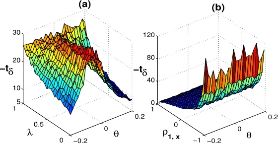
Remark 1 Where only one break exists, the asymptotic t-statistic associated withδˆin equation (2) is:
T−12tˆ δ
p
→ −
q
σ2u(1−ρ1x)
2[µ2x+θx(1−λx)(2µx+θx)]+σx2(1+ρ1x),
where→p indicates convergence in probability andρ1xis the first autocorrelation
ofxt.
Figure 1.aclearly illustrates the implication of the formula of the asymptotic t-statistic associated with ˆδin equation (2): where the structural break is positive, the DF test decreases its power, the larger the size of the break and the smaller the break fraction. Furthermore, where the structural break is negative, the DF test decreases its power when there is an increase in the size of the break only when (µx<−θx); analogously, an increase in the break fraction biases the DF test toward the acceptance of the null hypothesis if (−2µx
θx <1). Similarly,
figure 1.bshows that positive autocorrelation decreases the power of the test, and negative autocorrelation biases the DF test toward the rejection of the null hypothesis. The Monte Carlo section will show that the problems such as an increase in autocorrelation, the size and location of the breaks can be overcome by increasing the sample size.
3
A Monte Carlo study
−0.2 0
0.2
0 0.5 1
5 10 20 30
−0.2 0
0.2
−1 0 1 0 40 80 120
−tδ
θ θ
δ
−t
(a) (b)
[image:6.595.182.462.128.278.2]λ ρ1, x
Figure 1: t–statistic behavior according to the size and location of the break, and the degree of autocorrelation in the noise
theoretical results obtained in the previous section: firstly, columns 2 and 3 exemplify the effect of autocorrelation. The only difference between the DGPs in these two columns is that the first usesi.i.dinnovations whereas the second uses an stationaryAR(1) process. It is clear that rejection rates decrease in the presence of positive autocorrelation. Secondly, columns 4 and 5 illustrate that with an smaller positive break, rejection rates are greater, in the case of small sample sizes at least; and thirdly, columns 6 and 7 show the location of the break effect. With a positive break, the smaller the break fraction, the smaller the rejection rates.
T DGP1 DGP2 DGP3 DGP4 DGP5 DGP6
25 0.83 0.03 0.26 0.00 0.17 0.92
50 0.99 0.07 0.93 0.00 0.88 0.99
100 1.00 0.26 1.00 0.18 1.00 1.00
250 1.00 0.97 1.00 1.00 1.00 1.00
500 1.00 1.00 1.00 1.00 1.00 1.00
Table 1: Monte Carlo Experiment
The values of the parameters in the DGPs are as follows: All DGPsσǫ= 0.02, µx= 0.05
DGP1:λ1= 0.25λ2= 0.75θ1= 0.09θ2=−0.09ρx= 0 DGP2:λ1= 0.25λ2= 0.75θ1= 0.09θ2=−0.09ρx= 0.9
[image:6.595.154.457.469.550.2]4
Empirical evidence
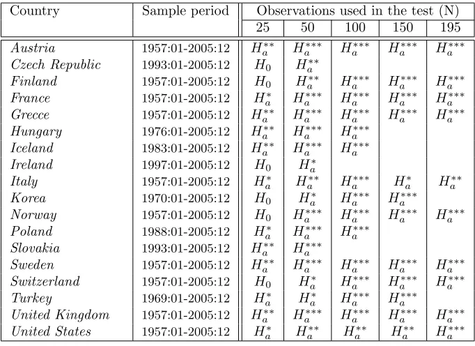
Theoretical results discussed earlier are illustrated by way of an empirical ap-plication; we analyze the results of the DF test applied to inflation rate series corresponding to the 30 OECD countries. Quarterly inflation rate series2 were constructed from monthly Consumer Price Index data retrieved from the In-ternational Monetary Fund’s InIn-ternational Financial Statistics data; the data span for these countries varies, the maximum sample period being 1957:01 to 2005:12.
Results of the DF test—with a constant, time trend and one lag3—shown in Table (2) attest the asymptotic properties of the DF test. For all the countries presented in this table (except Italy), evidence in favor of broken mean station-arity is stronger the larger the sample size. It is important to notice that the DF tests were performed to allow for first order autocorrelation only—we de-cided to use the specification studied in our asymptotic results, in the kowledge that the tests could suffer a consequent from loss of power4, nevertheless, in several cases, the null is rejected for sample sizes as small as 25. As shown in the Monte Carlo section, rejection rates found empirically are high for sample sizes of practical interest.
5
Conclusions
Structural breaks do affect the performance of UR tests. Nevertheless, we have shown the robustness of the DF test in the presence of structural breaks where the DGP of the series under analysis is mean stationary with breaks. In that case the t–statistic of the DF test diverges at rate√T implying that the null will, at some point, be rejected. However, our asymptotic results prove that the DF test is sensitive not only to the size of breaks, but also to their sign and their location, as well as to autocorrelation.
Monte Carlo experiments and empirical evidence show that the DF test provides adequate results when the sample size is sufficiently large. In fact, the DF is more sensitive to the presence of autocorrelation, regardless of the type of the break, although this phenomenon can also be alleviated by increasing the size of the sample or simply by running an Augmented DF test. UR testing can be reliably performed using a simple DF test if the sample size is large enough. In the specific case of inflation rates, the alternative of broken mean stationarity
2
Quarterly inflation series were computed as the logged differences of CPI at three-monthly intervals. For Australia and New Zealand we have quarterly CPIs; the quarterly inflation series are the logged differences of successive quarters.
3
The test was also performed under different specifications (DF with intercept, as well as intercept and time trend), providing similar results. Due to space constraints, we report this specification only and a subsample of countries. The other results are available upon request.
4
Country Sample period Observations used in the test (N)
25 50 100 150 195
Austria 1957:01-2005:12 H∗∗
a Ha∗∗∗ Ha∗∗∗ Ha∗∗∗ Ha∗∗∗
Czech Republic 1993:01-2005:12 H0 Ha∗∗
Finland 1957:01-2005:12 H0 Ha∗∗ Ha∗∗∗ Ha∗∗∗ Ha∗∗∗
France 1957:01-2005:12 H∗
a Ha∗∗∗ Ha∗∗∗ Ha∗∗∗ Ha∗∗∗
Grecce 1957:01-2005:12 H∗∗
a Ha∗∗∗ Ha∗∗∗ Ha∗∗∗ Ha∗∗∗
Hungary 1976:01-2005:12 H∗∗
a Ha∗∗∗ Ha∗∗∗
Iceland 1983:01-2005:12 H∗∗
a Ha∗∗∗ Ha∗∗∗
Ireland 1997:01-2005:12 H0 Ha∗
Italy 1957:01-2005:12 H∗
a Ha∗∗ Ha∗∗∗ Ha∗ Ha∗∗
Korea 1970:01-2005:12 H0 Ha∗ Ha∗∗∗ Ha∗∗∗
Norway 1957:01-2005:12 H0 Ha∗∗∗ Ha∗∗∗ Ha∗∗∗ Ha∗∗∗
Poland 1988:01-2005:12 H∗
a Ha∗∗∗ Ha∗∗∗
Slovakia 1993:01-2005:12 H∗∗
a Ha∗∗∗
Sweden 1957:01-2005:12 H∗∗
a Ha∗∗∗ Ha∗∗∗ Ha∗∗∗ Ha∗∗∗
Switzerland 1957:01-2005:12 H0 Ha∗ Ha∗∗∗ Ha∗∗∗ Ha∗∗∗
Turkey 1969:01-2005:12 H∗
a Ha∗ Ha∗∗∗ Ha∗∗∗
United Kingdom 1957:01-2005:12 H∗∗
a Ha∗∗∗ Ha∗∗∗ Ha∗∗∗ Ha∗∗∗
United States 1957:01-2005:12 H∗
[image:8.595.135.476.123.371.2]a Ha∗∗ Ha∗∗ Ha∗∗ Ha∗∗∗ Table 2: Results of the Dickey-Fuller test with intercept, time trend and one lag. Note: the *, **, and *** denote statistical significance at the 10%, 5% and 1% level respectively.
may be understood as the existence of an inflation targeting regime with time-varying inflation targets.
A
Appendix
Proof of Proposition 1. We present a guide on how to obtain the order in probability of one of the four t-statistics appearing in proposition (1), by using the DF regression (2) for which ∆xt=PNi=1x θiDPit+uxt−uxt−1 where
DPi,t=DUi,t−DUi,t−1. The other three cases follow the same steps. Proof as such was provided with the aid ofMathematica 4.1 software. The corresponding codes are available athttp://www.ventosa-santaularia.com/VSG 06b.zip. We shall now describe the process involved in establishing the aforementioned proof. The DF regression equation shall be ∆xt = α+δxt−1+ut in ma-trix form: ∆X = X1β+u. The vector of OLS estimators is βb = (αb bδ)′ = (X′
1X1)−1X1′∆X, and thet-statistic of interesttbδ =δb
b
σ2
u(X1′X1)−221
−1/2 , where (X′
1X1)−221 is the 2nd diagonal element of (X1′X1)−1 andσb2u =T−1
PT t=1ub2t =
T−1PT t=1
∆xt−αb−bδxt−1
2
PT
t=1∆xt=Op(1) PTt=1(∆xt)2=Op(T)
PT
t=1xt−1=Op(T) PTt=1x2t =Op(T)
PT
t=1∆xtxt−1=Op(T) PTt=1xt−1·t=Op T2
PT
t=1∆xt·t=Op(T) PtT=1∆xt∆xt−1=Op(T) We can fill the matrix (X′
1X1) as well as the vector (X1′Y) and then compute the OLS parameter estimates β = (X′
1X1)−1X1′∆X and the t-statistic associated withδ. The program computes the asymptotics5.
References
Arize, A., J. Malindretos, and K. Nam(2005): “Inflation and Structural Change in 50 Developing Countries,”Atlantic Economic Journal, 33(4), 461– 471.
Bai, J., and S. Ng(2004): “A PANIC Attack on Unit Roots and Cointegra-tion,” Econometrica, 72(4), 1127–1177.
Basher, S. A., and J. Westerlund (2006): “Is there really a Unit Root in the inflation rate? More Evidence from Panel Data Models,” MPRA paper No 136.
Cavaliere, G., and R. Taylor (2006): “Testing for a Change in Persis-tence in the Presence of a Volatility Shift,”Oxford Bulletin of Economics and Statistics, 68(s1), 761–781.
Chiquiar, D., A. Noriega,andM. Ramos-Francia(2007): “A time–series approach to test a change in inflation persistence: the mexican experience,” Working Paper 2007-01, Banco de Mxico.
Culver, S.,andD. Papell(1997): “Is there a unit root in the inflation rate? Evidence from sequential break and panel data models,”Journal of Applied Econometrics, 12(4), 435–444.
Dickey, D., and W. Fuller (1979): “Distribution of the Estimators for Autoregressive Time Series with a Unit Root,” Journal of the American Sta-tistical Association, 74, 427–31.
Gregoriou, A., and A. Kontonikas (2006): “”Inflation Targeting and the Stationarity of Inflation: New Results from an ESTAR Unit Root Test”,”
Bulletin of Economic Research, 58(4), 309–322.
Hassler, U., and J. Wolters (1995): “Long Memory in Inflation Rates: International Evidence,” Journal of Business & Economic Statistics, 13(1), 37–45.
5
Kim, T., S. Lee, andP. Newbold(2004): “Spurious Regressions With Sta-tionary Processes Around Linear Trends,”Economics Letters, 83, 257–262. Kim, T., S. Leybourne, and P. Newbold (2004): “Behaviour of
Dickey-Fuller Unit-Root Tests Under Trend Misspecification,”Journal of Time Series Analysis, 25(5), 755–764.
Lai, K.(1997): “On the disparate evidence on trend stationarity in inflation rates: A Reappraisal,”Applied Economics Letters, 4(5), 305–309.
Monta˜n´es, A. (1997): “Level Shifts, Unit Roots and Misspecification of the Breaking date,” Economics Letters, 54, 7–13.
Monta˜n´es, A.,andM. Reyes(1998): “Effect of a Shift in the Trend Function on Dickey-Fuller Unit Root Tests,” Econometric Theory, 14, 355–363.
Monta˜n´es, A., and A. Sans´o(2001): “The Dickey-Fuller Test Family and Changes in the Seasonal Pattern,”Annales d’ ´Economie et de Statistique, 61, 73–90.
Noriega, A., and D. Ventosa-Santaul`aria(2006): “Spurious Regression Under Broken Trend Stationarity,”Journal of Time Series Analysis, 27, 671– 684.
Perron, P.(1989): “The Great Crash, the Oil Price Shock and the Unit Root Hypothesis,”Econometrica, 57, 1361–1401.
Phillips, P.(1986): “Understanding Spurious Regressions in Econometrics,”
Journal of Econometrics, 33, 311–340.
Phillips, P.,and Z. Xiao(1998): “A Primer on Unit Root Testing,”Journal of Economic Surveys, 12(5), 423–470.
Sollis, R. (2001): “US and UK Inflation: Evidence on Structural Change in the Order of Integration,” Working Paper, Department of Economics and Ireland Trinity College Dublin.