Face Recognition by Radial Basis Function Network
(RBFN)
Mrinal Kanti Dhar
Lecturer, Dept. of EEE Leading University
Bangladesh
Quazi M. Hasibul Haque
R & D Engineer, Television Department.
Walton Bangladesh
Md. Tanjimuddin
Lecturer, Dept. of EEE Leading University
Bangladesh
ABSTRACT
Face recognition technology using Radial Basis Function Network (RBFN) is an attractive solution for the researchers who are working on the field of machine recognition, pattern recognition and computer vision. The key challenge in the face recognition technology is to provide high recognition rate. In this paper, an efficient method has been presented for face recognition using principal component analysis and radial basis function. More specifically, principal component analysis has been used for feature extraction and radial basis function network has been used as a classifier to classify data as well as for recognition process.
Keywords
Face recognition, Principal component analysis, Artificial neural network, Radial basis function network.
1.
INTRODUCTION
In the field of image processing, pattern recognition, computer vision, and neural network, every researcher concentrates on human face recognition by machine from still and video images. For doing this task, researchers are facing some difficulties when real time identification is required. One of the difficulties is that face image is highly variable and another one is variability of sources [1]. Total face recognition is obtained by three steps. These steps are - preprocessing, feature extraction and finally classification and recognition [2].
In the first step of preprocessing step, reduction of noise, possible convolute effects of interfering system are carried out [2]. Next step is feature extraction that plays an important role to represent a face in face recognition system. Feature extraction is one of the special forms of dimensionality reduction. In feature extraction process, input data is transferred into a set of features i.e. the relevant information of the input which will be used to do the desired task [3]. In feature extraction process, many researchers have proposed different techniques, as feature extraction by principal component analysis, independent component analysis, and linear discriminant analysis [4]. One of the most successful techniques among them is principal component analysis for extracting feature and representing data [10]. It not only reduces the dimensionality of the image but also retains some of the variations in the image data and provides compact representation of a face image [4][6]. Principal component analysis (PCA) is a statistical tool to convert a set of observations of possibly co-related variable into a set of values of uncorrelated variable called Principal Component (PC) by using orthogonal transformation [6]. Here,the number of original variables is greater than or equal to the number of
neurons of the RBF neural network. This process also improves its generalization capabilities.
2.
Experiments on the AT & T Database
The AT&T database (formerly ‘The ORL Database of Faces’) contains 400 grayscale images of 40 persons. Each person has 10 images. The size of each image is 112x92 pixels, with 256 gray levels per pixel. Images of the individuals have been taken varying light intensity, facial expressions (open/closed eyes, smiling/not smiling) and facial details (glasses/no glasses). Images are in PGM format and were taken against a dark homogeneous background, with tilt and rotation up to 20o and scale variation up to 10%. Sample face images of a person are shown in figure 1..
2.1
1
stExperiment
In the first experiment, 200 images of 40 different persons have taken. Each person has 5 images. After training process, different levels of noise have been added with the 200 images and then taken as test images. Next, correctly classified images are counted and listed in a table. In addition, the error curves are given in experimental results.
2.2
2
ndExperiment
In this experiment, 5 images of an individual is kept for training and another 5 images of the same individual are kept for testing. Thus, the training data set contains 200 images of 40 different persons. Rest of the 200 images are kept in testing data set.
2.3
3
rdExperiment
In this experiment, 200 images of 40 different persons are taken for training. The remaining 200 images are added by different levels of noise and are taken as testing data set.
3.
Program Execution and Performance
Testing
3.1
1
stExperiment Result
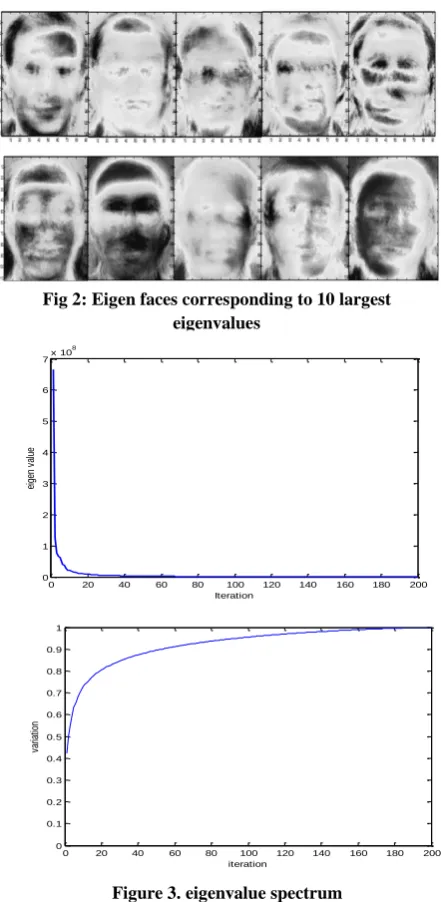
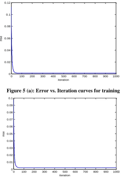
The eigenfaces corresponding to 10 largest eigenvalues are shown in figure 2. Figure 3 shows the eigenvalue plotted in descending form and eigenvalue spectrum in normalized form and how much variance the first n vectors account for.
[image:2.595.314.535.59.511.2]Fig 1: Sample images of a subject from the AT&T database
Fig 2: Eigen faces corresponding to 10 largest eigenvalues
0 20 40 60 80 100 120 140 160 180 200
0 1 2 3 4 5 6
7x 10
8
Iteration
ei
ge
n
va
lu
e
0 20 40 60 80 100 120 140 160 180 200
0 0.1 0.2 0.3 0.4 0.5 0.6 0.7 0.8 0.9 1
iteration
va
ria
tio
n
Figure 3. eigenvalue spectrum
[image:2.595.57.277.238.356.2]The error vs iteration curve for training and testing is shown in figure 4. Here no. of PCs = 80, no. of hidden neurons=120 and noise is zero.
0 100 200 300 400 500 600 700 800 900 1000 0
0.02 0.04 0.06 0.08 0.1 0.12 0.14
iteration
m
s
e
[image:2.595.334.535.568.713.2]The error vs iteration curve for training and testing is shown in figure 5 where no. of PCs = 80, no. of hidden neurons=120 and noise is zero mean with variance 0.002.
The error vs iteration curve for training and testing is shown in figure.6. Here no. of PCs = 80, no. of hidden neurons=120 and noise is zero mean with variance 0.008
0 100 200 300 400 500 600 700 800 900 1000 0
0.02 0.04 0.06 0.08 0.1 0.12 0.14
iteration
m
s
e
Figure 4(b): Error vs iteration curves for testing
0 100 200 300 400 500 600 700 800 900 1000 0
0.02 0.04 0.06 0.08 0.1 0.12
iteration
m
s
e
0 100 200 300 400 500 600 700 800 900 1000 0
0.01 0.02 0.03 0.04 0.05 0.06 0.07 0.08 0.09 0.1
iteration
m
s
e
Figure 5 (b): Error vs. Iteration curves for testing
0 100 200 300 400 500 600 700 800 900 1000 0
0.01 0.02 0.03 0.04 0.05 0.06 0.07
iteration
m
s
e
0 100 200 300 400 500 600 700 800 900 1000
0 0.02 0.04 0.06 0.08 0.1 0.12
iteration
m
s
e
Figure 6 (b): Error vs iteration curves for testing
0 100 200 300 400 500 600 700 800 900 1000 0
0.02 0.04 0.06 0.08 0.1 0.12
iteration
m
se
0 100 200 300 400 500 600 700 800 900 1000
0 0.01 0.02 0.03 0.04 0.05 0.06 0.07 0.08 0.09 0.1
iteration
m
se
Figure 7 (b): Error vs. iteration curves for testing Figure 6 (a): Error vs iteration curves for training
Figure 5 (a): Error vs. Iteration curves for training
[image:3.595.322.537.70.721.2] [image:3.595.55.258.73.214.2] [image:3.595.55.264.316.631.2].Network performance for 1st experiment is given below:
3.2
2
ndExperiment Result
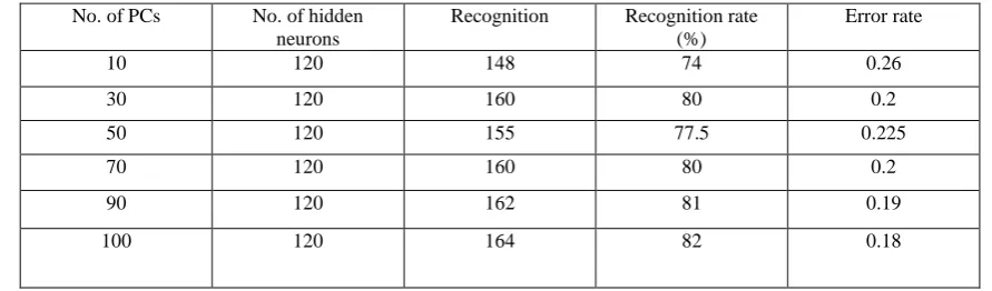
The error vs iteration curve for training and testing is shown in figure 7. Here no. of PCs = 80 and no. of hidden neurons=120. Network performance is observed after
performing this experiment for different number of PCs and hidden neurons. Here it is tabulated below in table 2
:
Best network performance is found for PC=80, hidden neuron=120 and PC=100, hidden neuron=140.
3.3
3
rdExperiment Result
The error vs iteration curve for training and testing is shown in figure.8. Here no. of PCs = 80, no. of hidden neurons=120 and noise is zero mean with variance .002
No. of PCs No. of hidden neurons
Noise Recognition Recognition rate (%)
Error rate
mean Variance
80 120 0 0 193 96.5 0.035
0 0.002 182 91 0.09
0 0.004 162 81 0.19
0 0.006 140 70 0.3
0 0.008 135 67.5 0.325
0 0.01 107 53.5 0.465
0.01 0.003 133 66.5 0.335
0.01 0.005 123 61.5 0.385
0.01 0.007 104 52 0.48
No. of PCs No. of hidden neurons
Recognition Recognition rate (%)
Error rate
10 120 148 74 0.26
30 120 160 80 0.2
50 120 155 77.5 0.225
70 120 160 80 0.2
90 120 162 81 0.19
100 120 164 82 0.18
No. of PCs No. of hidden neurons
Recognition Recognition rate (%)
Error rate
10 60 139 69.5 0.305
30 80 143 71.5 0.285
50 100 148 74 0.26
70 120 164 82 0.18
80 120 169 84.5 0.155
90 140 166 83 0.17
100 140 170 85 0.15
[image:4.595.81.518.118.259.2]Table 1: Network performance for different noise level
Table 2: Network performance for different no. of PCs
[image:4.595.73.519.364.495.2]The error vs iteration curve for training and testing is shown in figure.9. Here no. of PCs = 80, no. of hidden neuron=120 and noise is zero mean with variance 0.008.
This experiment is performed for different noise level and then network performance is observed. Table 4. Shows the network performance of 3rd experiment.
No. of PCs No. of hidden neurons
Noise Recognition Recognition rate (%)
Error rate
Mean variance
80 120 0 0.002 156 78 0.22
0.001 0.002 156 78 0.22
0 0.004 139 69.5 0.305
0.001 0.004 138 69 0.31
0 0.006 115 57.5 0.425
0 0.008 103 51.5 0.485
0 100 200 300 400 500 600 700 800 900 1000 0
0.02 0.04 0.06 0.08 0.1 0.12 0.14
iteration
m
s
e
0 100 200 300 400 500 600 700 800 900 1000 0
0.01 0.02 0.03 0.04 0.05 0.06 0.07 0.08 0.09 0.1
iteration
m
s
e
Figure 8 (b). Error vs iteration curves for testing
0 100 200 300 400 500 600 700 800 900 1000 0
0.02 0.04 0.06 0.08 0.1 0.12 0.14
iteration
m
s
e
0 100 200 300 400 500 600 700 800 900 1000 0
0.01 0.02 0.03 0.04 0.05 0.06 0.07
iteration
m
s
e
Figure 9 (b). Error vs. iteration curves for testing
Table 4: network performance for different noise level Figure 8 (a). Error vs. iteration curves for training
4.
Conclusion
In this paper, an effective method of face recognition technique has been presented. Image processing algorithms based on Radial basis function network has been used in this paper. This paper provides the application of PCA for feature extraction and RBF neural network for classification of face images as a classifier in the context of face recognition technology. It shows the proposed method performed pleasingly for all of the tested application domains. Even, this combination achieves a recognition rate of 96.5% with zero noise level. However, we have found some limitations too. Recognition rate falls badly as the noise level starts to increase. Therefore, researchers have scopes of works to minimize the noise effect. Introducing filtering networks and combining multi-type methods for feature extraction may increase the performance further.
5.
References
[1] Meng Joo Er, Shiqian Wu, Juwei Lu, Hock Lye Toh, “Face Recognition With Radial Basis Function (RBF) Neural Networks”, IEEE transactions on neural networks, vol. 13, no. 3, may 2002.
[2] V. Radha, N. Nallammal “Neural Network Based Face Recognition Using RBFN Classifier”, Proceedings of the World Congress on Engineering and Computer Science 2011 Vol I WCECS 2011, October 19-21, 2011, San Francisco, USA.
[3] L. Wang , X. Wang and J. Feng "On image matrix based feature extraction algorithms", IEEE Trans. Syst., Man, Cybern. B, Cybern., vol. 36, no. 1, pp.194 -197 2006
[4] Suganthy, M. and P. Ramamoorthy, “Principal Component Analysis Based Feature Extraction, Morphological Edge Detection and Localization for Fast Iris Recognition”, Journal of Computer Science 8 (9), pp.1428-1433, 2012
[5] Wang, Y., Jiar, Y., Hu, C., & Turk, M “Face recognition based on kernel radial basis function networks”. Asian Conference on Computer Vision, Korea. (2004, January 27-30).
[6] Lindsay I Smith “A tutorial on Principal Components Analysis” February 26, 2002.
[7] Powell, M. J. D, “Radial basis functions for multivariable interpolation:A review” In Algorithms for Approximation, J. C. Mason and M. G. Cox, Eds. Oxford University Press, Oxford, UK, 1987, pp. 143–167
[8] L.N.M.Tawfiq ,Q.H. Eqhaar, “ON RADIAL BASIS FUNCTION NEURAL NETWORKS”Journal of al-qadisiyah for pure science(quarterly). Vol-12, pages-12-18.
[9] Babu, R.V. Suresh, S. Makur, “A. ROBUST OBJECT TRACKING WITH RADIAL BASIS FUNCTION NETWORKS” IEEE international conference on Acoustics, Speech and Signal processing, 2007. Volume: 1, Page(s): I-937 - I-940.
[10]Aleix M. MartõÂnez, Avinash C. Kak, “A. ROBUST OBJECT TRACKING WITH RADIAL BASIS FUNCTION NETWORKS” IEEE Trans. Pattern Analysis and Machine Intelligence, vol. 23, no. 2, pp. 228-233, February 2001.
[11]Tiantian Xie, Hao Yu and Bogdan Wilamowski, “Comparison between Traditional Neural Networks and Radial Basis Function Networks”Industrial Electronics(ISIE), 2011 IEEE International Symposium on, pp. 1194-1199, Date of conference 27-30 June, 2011