Variations in Shape Context Descriptor: A Survey

Variations in Shape Context Descriptor: A survey

Neha Bhuptani

Computer Engineering Dept. Sardar Vallabhbhai Patel

Institute of technology, Vasad, Gujarat, India

Bjial Talati

HOD, Computer Engineering Dept., Sardar Vallabhbhai Patel

Institute of technology, Vasad, Gujarat, India.

ABSTRACT

There is a great significance of Image retrieval in multimedia and for image retrieval shape is one of the promising features. This paper presents a survey on one of the method of image retrieval based on shape. First, Shape context is described in this paper and the various versions of it that are implemented are given in detail. This paper gives a summarized view of all the methods of shape context in one single place. It investigates all the methods and gives a brief review. Shape context is descriptor that uses the global features of the shape.

General Terms

Feature Extraction, Image processing, Image retrieval.

Keywords

Shape Context, Content based image retrieval, Contour based methods, Object recognition.

1.

INTRODUCTION

Significant research efforts in providing tools for effective retrieval and organization of images catches the attention due to the increasing multimedia technology and the rapidly expanding image collections The necessity to find a desired image from a large collection is shared by many professional groups; including medical diagnosis, design engineers security check and crime prevention [1]. Content Based Image Retrieval or CBIR is the retrieval of these images based on visual features such as colour, texture and shape. CBIR is basically a two-step process which includes Feature Extraction and Image Matching (also known as feature matching).Feature Extraction is a process to extract image features to an apparent extent. This extraction process is performed on both query images and images in the database. Image matching involves using the features of both images and comparing them to search for similar features of the images in the database. CBIR does not consume the time wasted in manual annotation process of text based approach. This advantage has motivated researchers to employ a CBIR technique for research.

Shape is one of the most important feature and effective due to its relevance to human perception. Shape is all the geometric information that remains intact when location, scale, and rotation effects are filtered out from the object [2]. These shapes are represented by the descriptors. Descriptors are some set of numbers which are produced to describe a given shape. The shape may not be entirely reconstructable from the descriptors, but different shapes should have different descriptors such that the shapes can be discriminated. Efficient shape representation must follow some requirements like translation invariance, rotation invariance, scale invariance, and indentifiability, noise resistant and reliable [3].Automatic extraction of feature

vectors and real-time indexing should be computed efficiently.

The general shape description methods fall into two categories: Contour based and Region based proposed by MPEG7. Region based methods considers all the pixels within a shape region into consideration to obtain the shape descriptor. Region based methods are further divided into global and local region based methods. Global methods take the region as a whole into consideration during calculation. Local methods divide region into smaller parts called primitives and then accumulate the results together at the end. While contour based techniques exploit the contour information. Contour based methods are further divided into global and local contour based methods. They extract information only from the boundary of the shape and neglect the essential information contained in the shape interior [2].Global methods take contour as whole into consideration while the local methods breaks the contour into small parts called primitives. Examples of the contour based type include chain codes, Fourier descriptors, simple geometric border representations (curvature, bending energy, boundary length, and signature), shape context and examples of the region based include Euler number, area, eccentricity, elongatedness.

Global contour shape representation techniques usually compute a multi-dimensional numeric feature vector from the shape boundary information. Metric distance such as Euclidean distances used for matching between shapes. Point (or point feature) based matching is also used in particular applications [4].

Shape context is one of the contour based global descriptor. Due to its robustness to rotation and scaling and its effectiveness in object recognition, shape context (SC)is employed as the global shape feature.In this paper, shape context is explained in detail and reviews of various improvements done in shape context are given.

In this paper Section 2 describes global shape descriptor Shape context. Section 3 explains various improvements and variations done in shape context till now. Finally section 4 draws the conclusion and future work.

2.

SHAPE CONTEXT

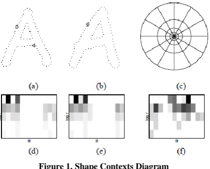
In [5], Belongie et al. describes the shape contexts descriptor. It indicates the coarse distribution of the rest of the shape with respect to a given point on the shape. The shape context descriptor of a given point on the shape is the histogram of the polar coordinates relative to all other points.

30

Figure 1. Shape Contexts Diagram

A shape context is a histogram that counts the number of sampled points along with their orientation and distance with respective to a reference point [6].

The descriptor can be given by [5]:

ℎ𝑖 𝑘 = # 𝑞 ≠ 𝑝𝑖: 𝑞 − 𝑝𝑖 ∈ 𝑏𝑖𝑛 𝑘 (1)

In this case, as shown in figure 1, the distance, log r, is divided into 5 bins and the degree of the orientation, θ, is divided into 12 bins. In Fig. 1(d)(e)(f) shows shape contexts with respective to the reference points marked by ○, ◊, Δ respectively. In Fig. 1(d)(e)(f), a large value bin is represented as a dark block.

It can be seen that the shape contexts of Fig.1 (d) and Fig. 1(e) are similar, because both represents the relatively similar points on two shapes. Due to similarity in shapes, the corresponding points on two different shapes will have similar shape context. On the other hand, the shape context is dependent on the orientation and size of a shape.

In [5], the shape contexts matching approach consists of three stages:

Step 1: Firstly the correspondence problem between the two shapes is solved by shape contexts descriptor and bipartite matching method.

Step 2: The correspondences is applied to estimate an aligning transform and use thin plate spline (TPS) modelling transformation and

Step 3: The distance between the two shapes as a sum of matching errors is computed.

The total cost of matching is minimized by Hungarian method. This method is used to solve the problem of bipartite graph matching and that can be done in a mass of time complexity: O(N3) [6].

Consider a point pi on the first shape P and a point qj on the second shape Q. The cost of matching between two points pi and qj is denoted by C ( pi,qj)and is computed by using the χ 2 test statistic as given in [8] is formulated in Eq. (2) which is given as follows:

𝐶 𝑝𝑖, 𝑞𝑗 =

1 2

ℎ𝑖 𝑘 − ℎ𝑗 𝑘 2

ℎ𝑖 𝑘 + ℎ𝑗 𝑘 𝐾

𝑘=1

2

The numbers of bins are decided such that they are uniform in log polar space. This will help in making descriptor more

sensitive to points nearby a particular point [7]. The shape context descriptor has the following invariance properties as mentioned in [3]:

 Translation: It is inherently translation invariant because it is calculated with the help of relative point locations.

 Scaling: Normalizing the radial distances by mean distance between all point pairs helps in making scale invariant.

 Rotation: Rotation invariance is accomplished by rotation of the coordinate system at each point in such that the positive x-axis is aligned with the tangent vector.

 Shape variation: It is robust against slight shape variations.

The two expensive steps in the above mentioned approach are: calculating the point correspondence between points of two shapes and calculating the cost matrix for matching the two shapes. Due to these steps, the major disadvantage of the above mentioned approach is that it is very computationally expensive. Hence it also not suited for large databases. So Many variations were done on in this method and survey of those methods is provided in this paper.

3.

VARIATIONS IN SHAPE CONTEXT

Shape context in a nutshell was shown in the above section. Now, this section focuses on the variations or improvements made in shape context to make it invariant to different transformations or make it computationally efficient or to make it work better for a particular set of datasets.

3.1

Generalized shape context:

This is an extension of the original version of the shape context. In original version, the central bins are smaller than those in the periphery and hence are less precise about the points far away from the center. In [9], a descriptor is extended by using oriented edges. To each edge point qj, they

attach a unit length tangent vector tj that is the direction of the

edge at qj. In each bin, summation of the tangent vectors for

all points falling in the bin is done. The descriptor for a point pi is the histogram hi:

ℎ𝑖 𝑘 = 𝑡𝑗 𝑞𝑗∈𝑄

𝑤ℎ𝑒𝑟𝑒 = 𝑞𝑗 ≠ 𝑝𝑖, 𝑞𝑗− 𝑝𝑖 ∈ 𝑏𝑖𝑛 𝑘 (3)

Now, each bin will hold a single vector in the direction of the dominant orientation of edges in the bin. For comparison of two point descriptors, they convert the d-bin histogram to a 2d-dimensional vector viand normalize these vectors and

compare them using L2 norm:

𝑣𝑖=< ℎ1,𝑥𝑖 , ℎ𝑖1,𝑦 , ℎ𝑖2𝑥 , ℎ𝑖2,𝑦 , … . . , ℎ𝑖𝑑,𝑥, ℎ𝑖𝑑,𝑦> 4

𝑑𝐺𝑆𝐶 ℎ𝑖, ℎ𝑗 = 𝑣𝑖− 𝑣𝑗 ₂ 5

1. Fast pruning: A set of likely candidates are retrieved quickly from a large collection of shapes given an unknown 2D query shape, As a result two algorithms of representative shape context and shapeme are introduced. In the first method, representative shape contexts (RSCs), few shape contexts for the query shape are computed and then attempt to match using only those. The other method, shapemes, uses vector quantization. It reduces the complexity of the shape contexts from 60-dimensional histograms to quantized classes of shape pieces [9].

2. Detailed matching: Once a small set of candidate shapes are retrieved, perform a more expensive and more accurate matching procedure to find the best matching shape to the query shape as mentioned in original version of shape context or generalized shape context.

3.2

Inner Distance Shape Context (IDSC):

One of the drawbacks of original version of shape context was that it could not handle articulated shapes [10]. This drawback was overcome by this method.

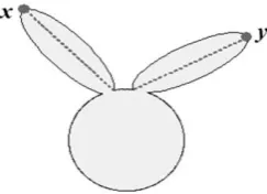
Figure 2. Shortest path between points x and y.

IDSC are descriptors that are robust to articulation and part structure. IDSC uses the concept of inner distance. Inner distance is defined as the length of the shortest path between landmark points within the shape. In technical words, two points x, y є O, their inner distance, denoted as d(x, y; O), is the length of the shortest path connecting x and y within O.In an example taken from [10], the dashed line shows the inner distance:

The inner distance can be calculated as:

To build a graph, treat each sample point pi as a node i in the

graph. Add an edge between node i and j, if and only if line segment pipjє O.

Apply to the graph any standard all-pair shortest path algorithms. Eg. Johnson or Floyd-Warshall’s algorithms, O(n3) complexity.

In IDSC, the Euclidean distance is replaced by inner-distance and relative orientation with the inner angle. This inner angle is defined as: Given two boundary points p, q and their shortest path Ґ(p,q;O), the angle between the contour tangent at p and the direction of Ґ(p,q;O) at p is the inner angle Ɵ(p,q; O) as shown in figure 3 [10]. Fig. 4 shows examples of the shape context which can be computed by the two different methods. It can be seen that SC is similar for all three shapes, while IDSC is only similar for the similar shapes. From this figure, it is clear that the inner-distance is superior at capturing parts in comparison to SC. But the drawback of inner distance is that it is sensitive to shape topology which sometimes causes problems.

Figure 3. The inner-angle Ɵ(p, q; O) between two boundary points.

Figure 4. Shape context (SC) and inner-distance shape context (IDSC).

3.3

Fast shape context using indexing

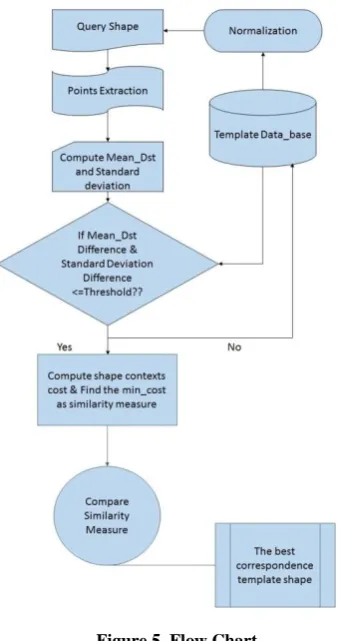
The Hungarian method used in original shape context is having high computational complexity. To reduce this complexity this method used mean distance and standard deviation of shape contexts as the index of shapes to reduce the matching candidates. Now, Best-fit Ellipse (BFE) modeling is used to normalize the size of the object as mean distance is dependent on shape’s size.

As shown in figure 5, firstly, the reference point is selected and mean of Euclidean distance and its standard deviation from other n-1 points is calculated. Now the query shape has one shape context while the training shapes contains the n shape context for each point as its points meanand standard deviation of shape context is need to be calculated. Now the threshold is selected for mean and standard deviation both. The shape context distance, Cij, between the query shape and each candidate shape context of a template shape is defined as:

𝐶𝑖𝑗= 𝐶 𝑝𝑖, 𝑞𝑗 =1₂

ℎ𝑖 𝑘 − ℎ𝑗 𝑘 2

ℎ𝑖 𝑘 − ℎ𝑗 𝑘 𝐾

𝑘=1

(6)

This method is scale invariant as normalization is done on the shapes. It is also rotation invariant [6].

3.4

Shapeme histogram descriptor

32

Figure 5. Flow Chart

The shape ℓ can thus be represented by a histogram coding the frequency of appearance of each of the k shapeme indices. By this means, they globally describe by a unique histogram SH each shape by applying the following equation:

𝑆𝐻 𝑥 = # 𝐼𝑖== 𝑥: 𝐼𝑖∈ 0, 𝑘 (7)

An example of the shapeme taken from [11] is shown in figure 6. The k means algorithm is used to cluster the shape context cluster space. It can be seen that at each of the points pi there is its corresponding index Ii, and the similar parts shared by both shapes are having same indices. Now the matching of the two shapes is reduced to find the k-NN in the space of shapeme histogram. The indexing structure that approximates K-NN search in sub linear time is proposed to efficiently retrieve those histograms.

3.5

FFT-RISC

The rotation invariance problem is solved in original version of shape context with high complexity. To overcome this problem, this variant of shape context was introduced. FFT-RISC solves the problem of this rotation invariance without

bringing in much complexity. This is a rotation-invariant shape context via FFT. In this method, a new pixel-level shape descriptor was proposed. This method include following steps:

Step 1: To calculate the feature matrix, first compute the shape context of each point on a shape S.

 Construct 2D histogram [hpq ]for each point p є S

where p =1,2,..M and q=1,2,..N and M and N are the dimensions of shape context as in orginal version of shape context..

 Normalize the histogram : hpqhpq /(L-1)

 Perform 2D FFT on histogram [hpq] which results in

new matrix [fpq].

 Now the feature matrix F(pi) =[ apq] where apq is the

modulus of fpq.

Step 2: After one gets the feature matrix for the shape, compute the point correspondence between two shapes P and Q. Initialize ѱ as an empty set.

 Initialize ѱ as an empty set.

 Compute the distance between two feature matrices F(Pi) and F(Qj)/

𝐷 = 𝑑𝑖𝑗= 𝑎𝑝𝑞𝑖 − 𝑏𝑝𝑞𝑗 2 𝑁

𝑞=1 𝑀

𝑝=1

𝑖 = 1,2, … , 𝐿 (8)

 Search (s,t)=argmin{dij}’ Add a new element (s,t) to

ѱ. Update D by removing the elements {dik|k=1,2,..,L} and {dkj| k=1,2,...L’}.

 If |ѱ| <L. Repeat step 2.

This application of 2D FFT solves the problem of high computational rotation invariance achievement in general shape context method. As the computation of FFT is very fast, it can be considered that the mentioned shape descriptor implemented by FFT does not lead to obviously higher computing cost in contrast to the original Shape Contexts [12].

4.

CONCLUSION AND FUTURE

DIRECTION

In this paper, discussion of several variations of shape context algorithm is made. Shape context algorithm is a histogram of the polar coordinates relative to all other points. First, the original shape context was shown. Then after, many variations were show. Each variation tries to improve the original shape

context. Firstly, generalized shape context reduces the computational expenses. Second method IDSC makes it possible for shape context to handle the articulated shapes. Third, shape context using indexing makes it fast. And fourth shapeme makes it possible shape context’s application to huge databases which contains large amount of images. Fifth, FFT RISC makes it rotation invariant with less complexity. Thus distinct shape context methods have different benefits. In spite of these variations, a focus is made on the research in shape context to make it more efficient and computationally inexpensive. Advantage of different variations can be combined to improve the accuracy and efficiency of the algorithm.

5.

REFERENCES

[1] Khokher, Amandeep, and Rajneesh Talwar. "Content-based Image Retrieval: Feature Extraction Techniques and Applications." In Conference proceedings. 2012.

[2] Pooja, Chandan Singh. "An Effective Image Retrieval System using Region and Contour based Features."

[3] Yang, Mingqiang, KidiyoKpalma, and Joseph Ronsin. "A survey of shape feature extraction techniques." Pattern recognition (2008): 43-90.

[4] Zhang, Dengsheng, and Guojun Lu. "Review of shape representation and description techniques." Pattern recognition 37, no. 1 (2004): 1-19.

[5] Belongie, Serge, Jitendra Malik, and Jan Puzicha. "Shape matching and object recognition using shape contexts." Pattern Analysis and Machine Intelligence, IEEE Transactions on 24, no. 4 (2002): 509-522.

[6] Lin, Chien-Chou, and Chun-Ting Chang. "A Fast Shape Context Matching Using Indexing." In Genetic and Evolutionary Computing (ICGEC), 2011 Fifth International Conference on, pp. 17-20. IEEE, 2011 [7] Schlosser S., and Beichel, R. “Fast Shape Retrieval

Based on Shape Contexts” In Image and Signal Processing and Analysis, 2009. ISPA 2009.

[8] Ma, Tian-lei, Yun-peng Liu, Ze-lin Shi, and Jian Yin. "A shape context based Hausdorff similarity measure in image matching." In ISPDI 2013-Fifth International Symposium on Photoelectronic Detection and Imaging, pp. 89070O-89070O. International Society for Optics and Photonics, 2013.

[9] Mori, Greg, Serge Belongie, and Jitendra Malik. "Efficient shape matching using shape contexts." IEEE Transactions on Pattern Analysis and Machine Intelligence 27, no. 11 (2005): 1832-1837.

[10] Ling, Haibin, and David W. Jacobs. "Shape classification using the inner-distance." Pattern Analysis and Machine Intelligence, IEEE Transactions on29, no. 2 (2007): 286-299.

[11] Rusiñol, Marçal, and JosepLladós. "Efficient logo retrieval through hashing shape context descriptors." In Proceedings of the 9th IAPR International Workshop on Document Analysis Systems, pp. 215-222. ACM, 2010.