Max–Planck–Institut f ¨ur biologische Kybernetik
Max Planck Institute for Biological Cybernetics
Technical Report No. TR-173
Example-based Learning for
Single-Image Super-Resolution
and JPEG Artifact Removal
Kwang In Kim
1and Younghee Kwon
2August 2008
1
Example-based Learning for Single-Image
Super-Resolution and JPEG Artifact Removal
Kwang In Kim and Younghee Kwon
Abstract. This paper proposes a framework for single-image super-resolution and JPEG artifact removal.
The underlying idea is to learn a map from input low-quality images (suitably preprocessed low-resolution or JPEG encoded images) to target high-quality images based on example pairs of input and output images. To retain the complexity of the resulting learning problem at a moderate level, a patch-based approach is taken such that kernel ridge regression (KRR) scans the input image with a small window (patch) and produces a patch-valued output for each output pixel location. These constitute a set of candidate images each of which reflects different local information. An image output is then obtained as a convex combination of candidates for each pixel based on estimated confidences of candidates. To reduce the time complexity of training and testing for KRR, a sparse solution is found by combining the ideas of kernel matching pursuit and gradient descent. As a regularized solution, KRR leads to a better generalization than simply storing the examples as it has been done in existing example-based super-resolution algorithms and results in much less noisy images. However, this may introduce blurring and ringing artifacts around major edges as sharp changes are penalized severely. A prior model of a generic image class which takes into account the discontinuity property of images is adopted to resolve this problem. Comparison with existing super-resolution and JPEG artifact removal methods shows the effectiveness of the proposed method. Furthermore, the proposed method is generic in that it has the potential to be applied to many other image enhancement applications.
1
Introduction
Single-image super-resolution and JPEG artifact removal are important yet unsolved problems. This paper pro-poses a method for these problems which can be possibly extended to many other image enhancement applications. The basic idea is to pose image enhancement as a regression problem and learn a function which maps input low-quality images to target images based on suitable pairs of example images. Then, the remaining problems are 1. to find a suitable representation of input images depending on the given class of problem which facilitates the subsequent learning; 2. to exploita prioriknowledge of a generic image class such that the errors occurring at the learning stage can be compensated; and 3. to find a solution which can deal with a large amount of data.1
This paper is organized as follows. The remainder of this section surveys single-image super-resolution, JPEG artifact removal, and existing methods for these problems, and motivates our regression-based approach. Section 2 and 3 discuss the above-mentioned sub-problems and develop the image super-resolution and the JPEG artifact removal algorithms, respectively. Experimental results are presented in Sect. 4 and conclusions given in Sect. 5.
1.1 Single-image super-resolution
Image super-resolution refers to the task of constructing high-resolution enlargements of low-resolution images. In contrast toimage interpolation(e.g., [1, 2]), new high-resolution details are added to the reconstruction. This prob-lem is inherently ill-posed as there are generally multiple high-resolution images that can be reduced to the same low-resolution image. Existing effort to resolve this problem resulted in two different categories of applications. Firstly,aggregation from multiple images[3, 4, 5, 6, 7, 8] assumes the existence of multiple images of asceneand aggregates the information spread around these images to produce a single high-resolution image. This requires estimating the registration parameters for aligning the low-resolution images, determining the characteristics of the sensor (e.g., point spread function (PSF)), and exploitinga prioriinformation of the image class to regularize the
1It should be noted that for many image enhancement problems, it is easy to generate a large set of example-image pairs: one
solution. Accordingly, multiple-image super-resolution research is mainly focused on solving these sub-problems [4, 5, 6, 7].
Conversely,single-image super-resolutionworks based on only a single image. In comparison to the multiple image case, this problem is even more severely underconstrained as less information about the scene is provided. Furthermore, single-image super-resolution can be more general as it might include magnifying images which do not have underlying ground truth (e.g., for the case of enlarging computer graphic images).2 In this case,
estimating sensor characteristics might be less meaningful and the objective becomes the generation of visually plausible images rather then reconstructing the underlying scene. Accordingly, for single-image super-resolution, one has to inevitably rely on very strong prior information. This prior information is available either in the explicit form of a distribution or energy functional defined on the image class [9, 10, 11, 12, 13, 14], and/or in the implicit form of example images which leads to example-based super-resolution [6, 15, 16, 17, 18, 19].
Previous example-based super-resolution algorithms can roughly be characterized as nearest neighbor (NN)-based estimation [6, 15, 16, 17, 19]: during thetraining phase, pairs of low-resolution and corresponding high-resolution image patches (sub-windows of images) are collected. Then, in thesuper-resolution phase, each patch of the given low-resolution image is compared to the stored low-resolution patches, and the high-resolution patch corresponding to the nearest low-resolution patch and satisfying a certain spatial neighborhood compatibility is selected as the output. For instance, Freeman et al. [15] posed the image super-resolution as the problem of estimating high-frequency details by interpolating the input low-resolution image into the desired scale (which results in a blurred image). Then, the super-resolution is performed by the NN-based estimation of high-frequency patches based on the corresponding patches of input low-frequency image and resolving the compatibility of output patches using a Markov network.
Baker and Kanade [6] represented images based on the Laplacian pyramid and estimated each pixel in high-resolution image using an NN search enforcing the consistency of the gradients around the pixel of interest. Similar algorithms were also derived as a special instance of image analogies[17] and in the context of maximum a posteriori(MAP) framework [19].
Although NN-based methods have already shown impressive performance, there is still room for improvement if one views the image super-resolution as a regression problem, i.e., finding a mapf from the space of low-resolution image patchesX to the space of target high-resolution patches Y. It is well known in the machine learning community that NN-based estimation suffers fromoverfittingwhere one obtains a function which explains the training data perfectly yet cannot be generalized to unknown data. This becomes prominent when the target function is highly complex or the data is high-dimensional [20], which is the case for image super-resolution. Accordingly, it is reasonable to expect that NN-based methods can be improved by adopting learning algorithms withregularizationcapability to avoid overfitting.
Indeed, attempts have already been made to regularize the estimator. Chang et al. [21] represented the input and target image patches with linear combinations of stored training patches, assuming that the patches in low-and high-resolution images form manifolds with similar local geometries to each other. Super-resolution is then performed by firstly finding a set of nearest low-resolution patches for an input low-resolution patch and recon-structing the input patch as a linear combination (calculated from locally linear embedding (LLE)) of the retrieved patches. Then, an output patch is obtained as the linear combination of the corresponding stored high-resolution patches using the combination coefficients of low-resolution patches (i.e., the LLE coefficients calculated from re-constructing a low-resolution patch are used to reconstruct the corresponding high-resolution patch). This method demonstrated an improved performance over the original NN-based method [21]. However it is not completely clear whether the assumption of a similar local geometry between low- and high-resolution image spaces is always satisfied.
A rather straightforward approach would be to regularize the regressor directly. Based on the framework of Freeman et al. [15, 16], Kim et al. [22] has posed the problem of estimating the high-frequency details as a regression problem which is then resolved by support vector regression (SVR). Meanwhile, Ni and Nguyen [23] utilized SVR in the frequency domain and posed the super-resolution as a kernel learning problem. While SVR produced a significant improvement over existing example-based methods, it has several drawbacks in building a practical system: 1. SVR synthesizes the outputs inRN (Nis the output patch size) which do not necessarily lie in
the set of realistic image patches. As a regularization framework, SVR tends to smooth sharp edges and produce an oscillation along the major edges (ringing artifacts). This might lead to low reconstruction error on average, but is visually implausible; 2. SVR results in a dense solution, i.e., the regression function is expanded in the whole set of
2
training data points and accordingly is computationally demanding both in training and in testing: optimizing the hyper-parameters based on cross-validation indicated that the optimum value offor the-insensitive loss function of SVR is close to zero [22].
The current work extends the framework of Kim et al. [22, 24]. Kernel ridge regression (KRR) is utilized in place of SVR. Due to the observed optimality ofat (nearly) 0 for SVR in our previous study, the only difference between SVR and KRR in the proposed setting is the use ofL1orL2-loss, respectively. TheL2-loss adopted by KRR is differentiable and facilitates gradient-based optimization.3To reduce the time complexity of KRR, a sparse solution is found by combining the idea of the kernel matching pursuit (KMP) [26] and gradient descent such that the time complexity and the quality of super-resolution can be traded. As the regularizer of KRR is the same as that of SVR, the problem of oscillation along the major edges still remains. This is resolved by exploiting a prior over image structure which takes into account the discontinuity of pixel values across edges (cf. Sect. 2.3).
1.2 JPEG Artifact Removal
Block-wise discrete cosine transform (DCT) coding has been successfully employed in image and video compres-sion applications, including the Joint Photographers Expert Group (JPEG) image comprescompres-sion and Motion Pictures Expert Group (MPEG) video compression standards. The basic idea is to divide the image (or video frames) into disjoint blocks and then individually transform, quantize, and encode each block. This approach well exploits ef-fectiveness of the DCT for the compression of small image blocks and its efficiency in hardware implementations. However, at low bit rates, decoded images exhibit block artifacts (discontinuities that appear between the bound-aries of the blocks) and ringing artifacts [27]. This problem can be resolved either by adopting a coding method with better compression capability (e.g., JPEG2000, learning-based methods [28]) or by post-processing the given compressed image to reduce the artifacts. The latter case might have more applicability as it can be applied to images which are compressed already and are not available in the uncompressed form.
There are several approaches for this problem. One of the most well-known method is the re-application of JPEG [29]. This method re-applies JPEG encoding to the shifted versions of already encoded image, shifts back the resulting images to the original position, and forms an average. The motivation behind this simple algorithm is the low-pass filtering properties of JPEG encoding within each quantization block, which when applied to shifted images, has effect of reducing the magnitude of blockiness. Despite its simplicity, the algorithm provided superior performance over many other existing methods (cf. references appearing in [29]).
As in other fields of image enhancement, utilizinga priori information of image class is essential in JPEG artifact removal. Penalizing total variation (TV) turned out to be a good candidate. Alter et al. [30] proposed weighting the degree of TV penalization depending on the complexity of region of interest (adapted TV) such that block boundaries are penalized more, while texture-areas are less-penalized. This is then actually resolved by iteration throughprojection onto convex sets[30]. The authors provided asymptotic proofs of convergence. However, they demonstrated that in practice, only a few steps (≈ 10) are enough to produce visually plausible results, and showed improvement over the re-application of JPEG.
Figure 1: Overview of super-resolution shown with an example: a. input image is interpolated into the desired scale, b. a set of candidate images is generated as the result of regression, c. candidates are combined based on estimated confidences; The combined result is sharper and less noisy than individual candidates, which however shows ringing artifacts, and d. post-processing removes ringing artifacts and further enhances edges.
2
Regression-based Image Super-resolution
Adopting the framework of Freeman et al. [15, 16], for the super-resolution of a given image, we estimate the corresponding missing high-frequency details based on interpolation into the desired scale (X), which in this work is obtained by the the cubic spline interpolation (henceforth referred to as ’interpolation’). Furthermore, based on the conditional independence assumption of high- and low-frequency components given band-frequency components of an image [16], the estimation of high-frequency components is performed based on the Laplacian of the interpolationX. The estimate can then be added to the interpolation to produce the super-resolved image. However, instead of generating a single image at once, we firstly generate a set of candidate estimates (Z). Each candidate is obtained based on different local observation of input image and accordingly contains different partial information of the underlying high-resolution image. A single high-resolution image is then obtained as a convex combination for each pixel of the set of candidate pixels based on their estimated confidence. To enhance the visual quality around the major edges, the results are post-processed based on the prior of natural images proposed by Tappen et al. [9]. Figure 1 summarizes the super-resolution process.
2.1 Regression
Using the notationNG(S(x, y))to represent aG-sized square window (patch) centered at the location(x, y)of
the imageS, the proposed method estimates the values ofY at specific locationsNN(Y(x, y))based on only the
values of (the Laplacian of)Xat corresponding locationsNM(X(x, y)).
Then, during the super-resolution,X is scanned with a patch (of sizeM (√M ×√M)) to produce a patch-valued regression result (of size N) for each pixel. As the patches are overlapping with their neighbors, this results in a set of candidate pixels for each location ofZ, which are then combined to make the final estimation (details will be provided in Sect. 2.2). The training patch pairs are randomly sampled from a set of low-resolution and corresponding desired high-resolution images (cf. Sect. 4.1.1). To avoid that the learning is distracted by uninformative patterns, the patches whose (Laplacian) norms are close to zero are excluded from the training set. Furthermore, to increase the efficiency of the training set, the data are contrast-normalized [16]: during the construction of the training set, both the input patch and corresponding desired patches are normalized by dividing them by the L1-norm of the input patch. For an unseen image patch, the input is again normalized before the regression and the corresponding output is inverse normalized.
3It is also possible to replace theL1
For a given set of training data points{(x1,y1), . . . ,(xl,yl)} ⊂ X ×Y ⊂RM×RN, we minimize the following
regularized cost functional for the regressorf ={f1, . . . , fN}:
O(f) =1 2
X i=1,...,N
X j=1,...,l
(fi(xj)−yji)
2+λkfik2 H
, (1)
whereyj = [yj1, . . . , y N
j ]andHis areproducing kernel Hilbert space(RKHS). Due to the reproducing property,
the minimizer of above functional is expanded in kernel functions:
fi(·) = X
j=1,...,l
aijk(xj,·), fori= 1, . . . , N, (2)
wherekis thereproducing kernel[32] forH, e.g., to be a Gaussian kernel
k(x,y) = exp
−kx−yk
2
σk
.
Equation (1) is the sum of individual convex cost functionals for each scalar-valued regressor and can be minimized separately. However, by tying the regularization parameterλand the kernelkwe can reduce the time complexity of training and testing down to the case of scalar-valued regression, as in this case the evaluations of kernel functions can be shared: plugging (2) into (1) and noting the convexity of (1) yields
A= (K+λI)−1Y, (3) whereY = [y>
1, . . . ,yl>]>,[K(i,j)]l,l = k(xi,xj), and thei-th column ofAconstitutes the coefficient vector
ai= [ai
1, . . . , ail]>for thei-th regressor.
The main difficulty in building a practical super-resolution system based on KRR (or SVR with close to zero) is its time complexity. As evident from (2) and (3), the training and testing time of KRR is O(l3) and
O(M×l), respectively, which becomes prohibitive even for a relatively small number of training data points (e.g.,
l ≈ 10,000). One way of reducing the time complexity is to trade it off with the optimality of the solution by finding the minimizer of (1) only within the span of asparsebasis set{k(b1,·), . . . , k(blb,·)}(lbl):
fi(·) = X
j=1,...,lb
aijk(bj,·), fori= 1, . . . , N.
In this case, the solution is obtained by
A= (KbxK>bx+λKbb)−1KbxY,
where[Kbx(i,j)]lb,l =k(bi,xj)and[Kbb(i,j)]lb,lb =k(bi,bj), and accordingly the time complexity reduces to
O(M ×lb)for testing. For a given fixedbasis pointsB={b1, . . . ,blb}, the time complexity of computing the
coefficient matrixAisO(lb3+l×lb×M). In general, the total training time depends on the method of findingB.
In KMP (withpre-fitting) [26], the basis points areselectedfrom the training data points in an incremental way: for givenn−1basis points, then-th basis point is chosen such that the cost functional (1) is minimized whenAis optimized accordingly. The original form of KMP does not include the regularization term (i.e.,λ= 0). However, augmenting KMP with regularization is straightforward. The exact implementation of KMP costsO(l2)-time for each step which leads toO(l2×l
b)complexity for the whole basis selection process.4Related algorithms can also
be found in [33, 34].5 Choosing a point from the training data set might result in a suboptimal solution if there
is no data points close to the desired basis points. If the data lies in a low-dimensional space and the training set is large enough, this effect is small and can be ignored. However, in high-dimensional spaces, the desired basis points might be far away from any data points [36].6
4
Here, we use the whole training set as candidates for being basis points.
5
Another commonly used basis selection approach is the linear programming (LP) boosting [35] where penalizingL1-norm of the expansion coefficient vector enforces sparsity. However, the regularizer used in LP boosting is different from those of (1) and accordingly is not directly comparable to the other methods considered here.
6As the sparse KRR is equivalent to the sparse Gaussian process (GP) regression, it can also be regarded as an instance of
Another possibility is to note the differentiability of the cost functional (1) which leads to gradient-based opti-mization toconstructB. Assuming that the evaluation of the derivative ofkwith respect to a basis vector takes
O(M)-time, which is the case for a Gaussian kernel:
∂
∂bk(x,b) =
2
σk
exp
−kx−bk
2
σk
(x−b)
= 2
σk
k(x,b)(x−b),
the evaluation of derivatives of (1) with respect toBand corresponding coefficient matrixAtakesO(M×l×lb+
l×l2
b):
7
∂
∂AO(f) = Kbx K
>
bxA−Y
+λKbbA
∂ ∂bi
O(f) = ∂Kbx(i,:)
∂bi
(K>bxA−Y)A(>i,:)+λ∂Kbb(i,:) ∂bi
AA>(i,:), fori= 1, . . . , lb. (4)
Because of the increased flexibility, in general, gradient-based methods can lead to a better optimization of the cost functional (1) than selection methods as already demonstrated in the context of sparse Gaussian process (GP) regression [37]. However, due to the non-convexity of (1) with respect toB, it is susceptible to local minima and accordingly a good heuristic is required to initialize the solution.
In this work, we use a combination of KMP and gradient descent. The basic idea is to assume that at then-th step of KMP, the chosen basis pointbn plus the accumulation of basis points obtained until the(n−1)-th step
(Bn−1) constitute a good initial search point. Then, at each step of KMP,Bncan be subsequently optimized by
gradient descent. Na¨ıve implementation of this idea is still very expensive. To reduce further the complexity, the following simplifications are adopted: 1. In the KMP step, instead of evaluating the whole training set for choosing
bn, onlylc(lc l) points are considered; 2. Gradient descent ofBnand correspondingA(1:n,:)are performed only at the everyr-th KMP step. Instead, for each KMP step, onlybnandA(n,:)are optimized. In this case, the gradient of (1) with respect tobncan be evaluated atO(M×l)-cost.8 Furthermore, similarly to [34], for a given
bnthe optimalA(n,:)can be analytically calculated at the same cost:
A(n,:)=
Kbx(n,:)
Y−K>bx(1:n−1,:)A(1:n−1,:)
−λKbb(n,:)A(1:n−1,:)
Kbx(n,:)K>bx(n,:)+λ
.
At then-th step, thelc-candidate basis points for KMP are selected based on a rather cheap criterion: we use the
distance between the function output obtained at the(n−1)-th step and an estimation of the response offullKRR
C(xk) = X
i
X j=1,...,n
aijk(bj,xk)−˜gi(xk)
2
, fork= 1, . . . , l,
where{˜gi}denotes an estimation of the full KRR which one might have obtained by training on allldata points,
and is calculated based onlocalized KRRs: for a given input x, its nearest neighbors (NNs) are collected in the training set and the full KRR is trained based on only these NNs. The output of this localized KRR forxthen constitute{g˜i(x)}. The candidate points are then chosen as the training data points corresponding to thel
c-largest
values ofC. It should be noted that the localized KRRs cannot be directly applied for regression as they might interpolate poorly on non-training data points. Once computed at the beginning,{˜gi(x
k)}is fixed throughout the
whole training process. For optimization, we used a conjugate gradient type algorithm9which locally approximates
the Hessian matrix at each step. To facilitate faster convergence, the Hessian is indirectly preconditioned by scaling
AandBsuch that average scales of them become the same to each other.
7
With a slight abuse of the Matlab notation,A(m:n,:) stands for the submatrix ofAobtained by extracting the rows ofA
frommton. Likewise,A(:,m)is defined as them-th column ofA.
8
It should be noted that[[Kbx]>n−1,l[A]n−1,N]l,N(cf. (4)) is stored at the(n−1)-th step. Accordingly, at then-th step,
augmenting a single row ofKbxandA, respectively is sufficient for calculating the gradient.
9
We used the code provided by Carl E. Rasmussen which is available athttp://www.kyb.tuebingen.mpg.de/
50 100 200 300 500 750 1000 40 50 60 70 80 90 100 110 120
# basis points
[image:8.612.187.415.51.225.2]Cost Random selection K−means Gradient descent KMP+gradient descent KMP
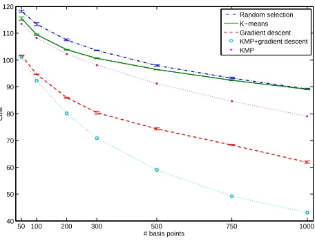
Figure 2: Performance of different sparse solution methods evaluated in terms of the cost functional (1) for the case of magnifi-cation factor 3 along each dimension; Details of experimental setups are described in Sect. 4.1; A fixed set of hyper-parameters were used for all cases such that the comparison can be made directly in (1). The performance of randomized algorithms (random selection, k-means, gradient descent) are calculated as averages of results from 20 different experiments with random initializations. The lengths of error bars correspond to twice the standard deviations.
To gain an insight into the performance of our basis construction method, a set of experiments has been per-formed with different sparse solution methods, including random selection (of basis points from the training set), KMP, means algorithm (clustering of training data points), na¨ıve gradient descent (with basis initialized by k-means), and the proposed combination of KMP and gradient descent, with 10,000 training data points.10 Figure 2 summarizes the results. All the basis selection and construction algorithms outperformed random selection of basis from training data points. The KMP showed an improved performance over the k-means algorithm which builds the basis set without reflecting the cost functional to be optimized. Except for k-means, the basis construction methods outperformed the basis selection method (KMP). The improved performance of combination of KMP could be attributed to the better initialization of the solution for the subsequent gradient descent step. It should be noted that the scales of error bars of randomized algorithms are relatively smaller than the differences between the average costs of all the algorithms. This indicates that the performance of the proposed method is unlikely to be achieved by performing random initialization plus gradient descent several times.
2.2 Combining Candidates
It is possible to construct a super-resolved image using only the scalar-valued regression (i.e.,N = 1) or patch-based regression with non-overlapping patches such that each pixel of Y (and accordingly Z) is reconstructed based on only the corresponding input patch ofX. However, we propose to predict a patch-valued output for each pixel such that overlapping patches provideNdifferent candidates for each pixel. These candidates constitutes a 3-D imageZwhere the third dimension corresponds to the candidates. This setting is motivated by the observation that 1. by sharing the hyper-parameters, the computational complexity of resulting patch-valued learning reduces to the scalar-valued learning; 2. the candidates contain information of different input image locations which are actually diverse enough such that the combination can boost the performance: in our preliminary experiments,11
constructing an image by choosing the best and the worst (in terms of the distance to the ground truth) candidates from each 2-D location ofZ resulted in an average peak signal-to-noise ratio (PSNR) difference of 7.84dB. Cer-tainly, the ground truth is not available at actual super-resolution stage and accordingly a way of constructing a single pixel out ofNcandidates is required.
One straightforward way is to construct the final estimation as a convex combination of candidates based on a certain confidence measure. For instance, by noting that the (sparse) KRR corresponds to the MAP estimation with the (sparse) GP prior [37], one could utilize the predictive variance as a basis for the selection. It is also possible
10
For this and all the other experiments in this paper, we set the size of intervalrand the number of candidate basis pointslc
to 10 and 100, respectively.
11
to learn the combiner and regressors simultaneously such that an error measure is minimized (e.g. mixture of expert setting [38]). In the preliminary experiments, both methods resulted in improvements over the scalar-valued regression. However, a better prediction was obtained when the confidence estimation is obtained based not only on the input patches but also on the context of neighboring reconstructions. For this, a set of linear regressors is trained such that for each location(x, y), they receive a patch of output images Z(NL(x,y),:) and produce the
estimation of differences ({d1(x, y), . . . , dN(x, y)}) between the unknown desired output and each candidate. The
final estimation of pixel value for an image location(x, y)is then obtained as the convex combination of candidates given in the form of asoftmax:
Y(x, y) = X
i=1,...,N
wi(x, y)Z(x, y, i),
where
wi(x, y) =
exp−|di(x,y)|
σC
P
j=1,...,Nexp
−|dj(x,y)|
σC
.
There are a few hyper-parameters to be tuned: for the regression part, the input and output patch sizes (M and
N, respectively), KRR parameters (σk andλ), and the number of basis points (lb) and for the combination part,
the input patch size (L) and the weight parameter (σC). We fixlb,N, andLat300,25(5×5), and49(7×7),
respectively. These values are determined by trading the quality of super-resolution off with the computational complexity. We observed constant increase of the performance as lb increases and becomes larger than300.
Similar tendency was also observed with increasingN(< M)andL while the run-time complexity increases linearly with all these parameters.
The remaining hyper-parameters are chosen based on error rates of super-resolution results for a set of validation images. However, directly optimizing these many parameters is computationally very demanding, especially due to the large time complexity of choosing basis points. With 200,000 training data points, training a sparse KRR for a given fixed parameters took around a day on a 3GHz machine (for the magnification factor 2 case; cf. Sect. 4.1 for details). To retain the complexity of the whole process at a moderate level, we firstly calculate a rough estimation of parameters based on a fixed set of basis points which is obtained from the k-means algorithm. Then, the full validation is performed only at the vicinity of the rough estimation. For the distance measure of k-means clustering, we use the following combination of Euclidean distances from both the input and output spaces which leaded to an improved performance (in terms of the KRR cost (1)) over the case of using only the input space distance:
d([xi, yi],[xj, yj]) = q
kxi−xjk2+ (σX/σY)kyi−yjk2,
whereσXandσY are variances of distances between pairs of training data points inX andY, respectively.12 It should be noted that the optimization of hyper-parameters for the regression and combination parts should not be separated: choosing the hyper-parameters of regression part based on cross-validation of regression data (pairs of input and output patches) leaded to much more conservative estimation (i.e.,σkandλare larger) than the
case of optimizing jointly the regression and combination parts. This can be explained by (further) regularization effect of the combination part which can be regarded as an instance of ensemble estimator. It has well known that in general, ensembles of individual estimators can lead to lower variances (expectation of variance of the output for a given set of training data points) and accordingly are smoother than individual estimators (Ch. 7 of [39] and references therein). This makes the optimization criteria a non-differentiable function of hyper-parameters and prevents us from using a rather sophisticate parameter optimization methods, e.g., gradient ascent of the marginal likelihood [37].
In the experiments, we focused on the desired magnification factors at{2,3,4}along each dimension (i.e., the number of pixels in the super-resolved image is{22,32,42}-times larger than that of the low-resolution image). Application to other magnification factors should be straightforward. Table 1 summarizes the optimized parame-ters. In this parameter setting, for the case of magnification factor 2, the combination of candidates resulted in an average PSNR increase of 0.46dB over the scalar-valued regression in the super-resolution results.
12
For a given kernel, an even better choice turned out to be reflecting the geometry of the space of the basis set to the distance measure:
d([xi, yi],[xj, yj]) =
q
kk(xi,·)−k(xj,·)k2H+ (σH/σY)kyi−yjk2.
Table 1: Parameters for super-resolution experiments
Mag. factor M σk σC λ σN TM1 TM2
2 7×7 0.05 0.04 0.5·10−7 127 2.2 0.95 3 9×9 0.011 0.17 0.1·10−7 80 2.2 0.5 4 13×13 0.006 0.12 0.5·10−7 70 1.1 1.0
2.3 Post-processing Based on Image Prior
As demonstrated in Fig. 4.b, the result of the proposed regression-based method is significantly better than the in-terpolation. However, detailed visual inspection along the major edges (edges showing rapid and strong change of pixel values) reveals smoothed edge boundary and ringing artifacts. In general, regularization methods (depending on the specific class of regularizer) including KRR and SVR tend to fit the data with a smooth function. Accord-ingly, at the sharp changes of the function (edges in the case of images) either edges are smoothed or oscillation occurs to compensate the resulting loss of smoothness. This might happen for all the levels of images demon-strating the discontinuity. However, the magnitude of oscillation is in proportion to the magnitude of changes and accordingly only visible at the vicinity of major edges. While this problem can indirectly be resolved by imposing less aggressive regularization at the edges, more direct approach is to rely on the prior knowledge of disconti-nuity of images. In this work, we use a modification of the natural image prior (NIP) framework proposed by Tappen et al. [9]:
P({x}|{y}) = 1
C
Y
(j,i∈NS(j))
exp
−
|ˆx j−xˆi|
σN α ·Y j exp " − xˆ j−yj
σR 2#
, (5)
where{y} represents the observed variables corresponding to the pixel values of Y,{x} represents the latent variable,NS(j)stands for the 8-connected neighbors of the pixel locationj, andCis a normalization constant.
With the objective of achieving the maximum probability (equivalently, the minimum energy as the inverse of (5)) for a given image, the second product term has the role of preventing the final solution flowing far away from the input regression-based super-resolution resultY, while the first product term (NIP term) tends to smooth the image based on the costs|xˆj−xˆi|. The role ofα(<1)is to re-weight the costs such that the largest difference is
stressed relatively less than the others and accordingly large changes of pixel values are relatively less penalized. Furthermore, the cost term|xˆj−xˆi|αbecomes piece-wise concave with boundary points (i.e., boundaries between
concave intervals) atNS(j)such that if the second term is removed, the minimum energy for a pixeljis achieved
by assigning it with the value of a neighbor, rather than a certain weighted average of neighborhood values which might have been the case whenα > 1. Accordingly, this distribution prefers a strong edge rather than a set of small edges and can be used to resolve the problem of smoothing around major edges. The optimization of (5) is performed by a max-sum type belief propagation (BP) similarly to [9]. To facilitate the optimization, we reuse the candidate set generated from the regression step such that the best candidates are chosen by the BP.
a b
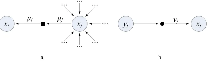
Figure 3: A node in the factor graph representation for the optimization of (5): a. NIP term and b. deviation penalty term; the message from the observation variable nodeyjto the factor node (solid circle) is a constant.
a b c d
[image:11.612.186.410.461.546.2]e f
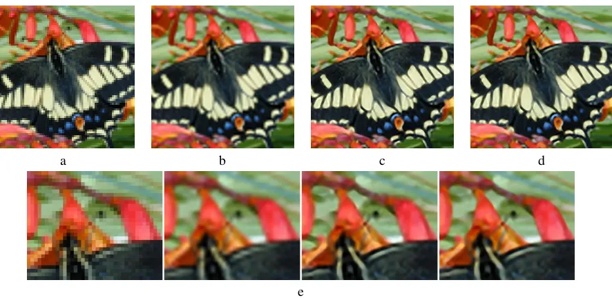
Figure 4: Example of super-resolution: a. interpolation, b. regression result, c. post-processed result of b based on NIP, d. Laplacian of interpolation with major edges displayed as green pixels, and e and f. enlarged portions of a-c from left to right.
logµi(xi) = max xi
logµj(xj)−
1 2
|xj−xi|
σN α
logµj(xj) = logνi(xj) + X k∈N(j)\i
logµk(xj)
logνj(xj) = −
1 2
|x j−yj|
σR 2
.
Optimizing (5) throughout the whole image region can lead to degraded results as it tends to flatten textured area.13 This problem is resolved by applying the modified NIP only at the vicinity of major edges. Based on the
observation that the input images are blurred and accordingly very high spatial frequency components are removed, the major edges are found by thresholding each pixel based on theL2 norm of the Laplacian and the range of pixel values in the local patches (i.e., classifying a pixel into ’major edge class’ if the norm of Laplacian and the maximum difference of pixel values within a local patch are larger than thresholdsTM1andTM2, respectively).14
It should be noted that the major edge is in general different from the object contour. For instance, in Fig. 4.d, the boundary between the chest of the duck and water is not detected as major edges as the intensity variations are
13
In original work of Tappen et al. [9], this problem does not happen as the candidates are2×2-size image patches rather than individual pixels.
14Here we define indirectly the major edges by a set of pixels which are in the local contexts of significant, nonlinear change
not significant across the boundary. In this case, no visible oscillation of pixel values are observed in the original regression result.
As it is evident from (5), in the energy minimization framework, only the relative scales of two product terms are important and accordinglyCandσRcan be held fixed at 1. Furthermore, we have observed that the roles ofσRand
α <1are similar to each other: as their values become smaller, the post-processing becomes more aggressive and raising the value of one parameter can roughly be compensated by lowering the value of the other. Accordingly, we also setαbeing fixed at 0.85. The remaining parametersσN,TM1, andTM2could be optimized in the same way to that of other hyper-parameters (cf. Sect. 2.2). However, we setσRvalue more aggressive than the optimal
solution (in terms of PSNR) as it produced visually much more plausible images.15 The obtained parameters for
the NIP are summarized in Table 1. While the improvements in terms of PSNR are not significant (e.g., for the case of magnification factor 2, on average 0.0003dB from the combined regression result) the improved visual quality at major edges demonstrate the effectiveness of using the prior of natural images (Fig. 4).
2.4 Processing Color Images
There can be many different ways to extend the gray image super-resolution algorithm for processing color images. One of the simplest ways is to process only the luminance component of a given color image as motivated by larger sensitivity of human eye for luminance component over the chrominance components [5, 21]. For this, the input image is firstly represented in YIQ color space and the super-resolution is performed only for the Y component. The final result is then obtained by combining the super-resolved Y component with the I and Q components of interpolated image. This scheme has important advantages of enabling the gray level model being applied directly to color images and resulting in the run-time complexity to be the same to that of gray level case. Another way to apply the gray model directly to color images is to regard each color channel as a gray level image. This results in improved performance over super-resolving only the luminance components both in PSNR values and in visual plausibility at the expense of 3 times larger run-time complexity. In general, statistical properties of each channel are different from each other. Accordingly, one might expect further improvement of performance by training separate models for each channel preceded by a proper decorrelation, or training a single large model which considers all color channels simultaneously. However, in our preliminary experiments, simultaneous learning did not show any visually noticeable improvement over the gray level learning case (there was an observable improvement of PSNR values, though). Accordingly, we propose to use one of the first two candidates in practice. Figure 5 shows an example of color image super-resolution.
3
Regression-based JPEG Artifact Removal
The idea of the proposed JPEG artifact removal method is to cast the problem into the super-resolution (i.e., estimating missing high-frequency details) by blurring the input JPEG image. Then, the remaining problem is to choose suitable blur kernels such that the subsequent super-resolution is facilitated. We adopt Gaussian blur as proposed in [27]. However, it should be noted that for textured regions, the degree of burring should be controlled to prevent losing the details. On the other hand, for rather flat regions (regions which do not show any significant change of pixel values), intense blurring might be desirable as the block artifacts are clearly visible there and there might be no significant loss of information occurred by blurring. Accordingly, we use two different blur kernels for flat regions and non-flat regions, respectively. To identify flat regions, we firstly blur the input JPEG image with a small width parameter (weak blurring) and calculate the Laplacian of resulting blurred image. Then, each pixel in the Laplacian is classified into flat class if the norm of a local patch encompassing that pixel is larger than a threshold. As we have not observed any significant improvement of visual quality by super-resolving flat regions, the super-resolution is performed only for the non-flat regions.
In principle, one could build a single large artifact removal model for JPEG images at various different com-pression factors. However, more economical approach might be to train a model specialized to each small range of compression factors. Then, removing artifacts of a given input JPEG image can be performed by choosing the proper model based on its compression factor which is determined by the quantization table stored at the header of JPEG file.
The parameters were optimized in the same way as the super-resolution case except for the additional three parameters which include widths of Gaussian kernels for flat regions (σF) and non-flat regions (σN F), plus the
15
All three parameters (σR,TM1, andTM1) are first optimized in terms of PSNR andTM1andTM2are held fixed at the
a b c d
[image:13.612.78.521.48.264.2]e
Figure 5: Example of color image super-resolution (magnification factor 4): a. nearest neighbor interpolation, b. spline interpolation, c. luminance component super-resolution: The result is significantly better than a and b; However, detailed visual inspection along the major edges (e.g., boundaries of flowers) reveals some blurring remaining (cf. e), d. separate super-resolution for each color channel (in RGB), and e. enlarged portions of a-d from left to right.
Table 2: Parameters for JPEG artifact removal experiments
Quantization table index [29] Q1 Q2 Q3
M 7×7 7×7 9×9
σk 0.045 0.027 0.012
σC 0.05 0.06 0.06
λ 0.5·10−7 0.1·10−7 0.1·10−7
σN 220 140 80
TM1 2.7 2.7 1.5
TM2 1.5 0.7 1.0
σF 0.8 1.1 1.35
σN F 0.9 1.4 2.7
TF 1.5 1.2 1.3
threshold (TF) used in determining the flat and non-float classes. To reduce the complexity of whole training
process, these three parameters were determined based on scalar-valued regression in the super-resolution. Once the parameters were obtained, they are held fixed during the subsequent training of super-resolution stage. Table 2 summarizes the parameters optimized for three different quantization tables (Q1-Q3; cf. Sect. 4.2 for details). Figure 6 shows an example of JPEG artifact removal.
4
Experiments
4.1 Super-resolution
4.1.1 Experimental Setup
[image:13.612.155.443.349.488.2]a b c d
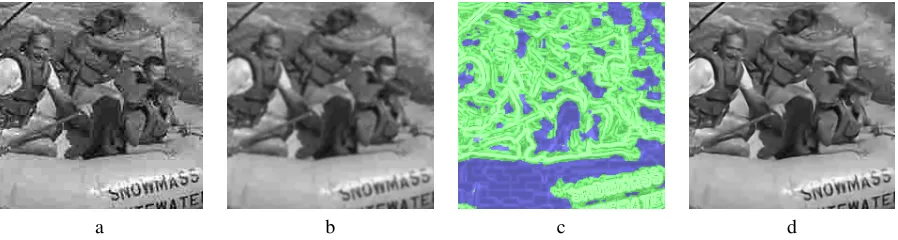
Figure 6: Example of JPEG artifact removal (Q2, cf. Sect. 4.2.1): a. input JPEG image, b. input image blurred withσN F, c.
[image:14.612.77.521.212.380.2]Laplacian of blurred image with non-flat regions displayed as green pixels, and d. final result.
Figure 7: Gallery of test images (disjoint from training images): we refer to the images in the text by its position in raster order. For super-resolution experiments, the lower-right corner of each image is truncated such that the size of each dimension becomes the multiple of the desired magnification factor.
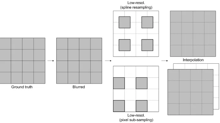
pixel as a weighted combination of high-resolution pixels (e.g., with spline interpolation (resampling)). We choose the latter setting as it is naturally unbiased to any specific direction (Fig. 8).
For comparison, several different example-based image super-resolution methods were implemented, which in-clude Freeman et al.’s fast NN-based method [16], Chang et al.’s LLE-based method [21], Tappen et al.’s NIP [9],16 and our previous SVR-based method [22] (trained based on only 10,000 data points). Experiments with Tap-pen et al.’s NIP were performed only at the magnification factor 2 as it was not straightforward to implement them for the other magnification factors. For the same reason, Freeman et al.’s NN method was applied only to the case of magnification factors 2 and 4. For comparison with non-example-based methods which are not implemented by us, we performed super-resolution on several images downloaded from the website of the authors of [11, 12, 15]. To obtain super-resolution results at image boundary, which are not directly available asM > N for the pro-posed methods and similarity for other example-based methods, the input images were extended by symmetrically replicating pixel values across the image boundary. For the experiments with color images, we applied the model trained on intensity images to each RGB channel and combined them.
4.1.2 Results
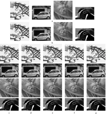
Figures 9 and 10 show examples of super-resolution. All the example-based super-resolution methods out-performed the nearest neighbor (NN)-interpolation and spline interpolation in terms of visual plausibility. The
16The original NIP algorithm was developed for super-resolving the pixel subsampled image. Accordingly, for the
Figure 8: Configuration of subsampling and ubsampling by interpolation for the case of magnification factor 2; Shaded squares represent actual pixel locations in low- and high-resolution images. Constructing a low-resolution image by pixel sub-sampling implies a specific directional preference in image generation process (lower left corner in the example; the third column); Actually pixel sub-sampling and spline resampling does not make any significant visual difference. However, the interpolation (and corresponding super-resolution) of a pixel sub-sampled image into the desired scale can result in sub-pixel displacements (the last column).
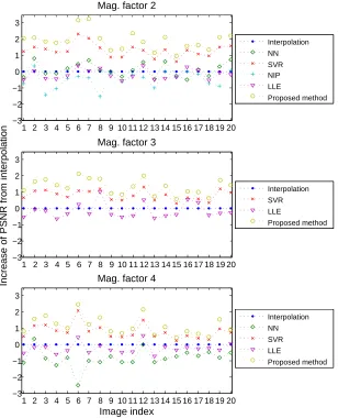
NN-based method and the original NIP produced sharper images at the expense of introducing noise which, even with the improved visual quality, lead to lower PSNR values than the interpolations (Fig. 11). The results of LLE are less noisy. However, it tended to smooth out texture details as observed in the third image of Fig. 9.e and accordingly produced low PSNR values. The SVR produced less noisy images and did not smooth out texture details. However it generated smoothed edges and perceptually distracting ring artifacts which have almost disap-peared in the results of the proposed method (e.g., the first image of Fig. 9.c). Disregarding the post-processing stage, we measured on average 0.60dB improvement of PSNRs for the proposed method from the SVR. This could be attributed to the sparsity of the solution which enabled training on a large data set and the effectiveness of the candidate combination scheme. Moreover, in comparison to SVR, the proposed method requires much less pro-cessing time: super-resolving a256×256-size image into512×512requires around 27 seconds for the proposed method and 18 minutes for the SVR-based method on a 3GHz machine. For quantitative comparison, PSNRs of different algorithms are plotted in Fig. 11.
An interesting property of NN-based method is that it introduced certain texture details which were absent in the input low-resolution images and even in the ground truth images. Sometimes, these ’pseudo textures’ provided more realistic images than others (e.g., the second image of Fig. 10.c). On the other hand, the proposed method did not generate such new texture details and instead provided a coherent enhancement of existing texture and edge patterns. As noted in [12] a preference between the two techniques may depend on the specific image and subjective concerns.
Figure 12 compares the proposed method with a non-example-based method proposed by Dai et al. [11] which combines the prior on the transition of pixel values across the edges and a metric induced by the graph cut al-gorithm.17 While both methods provided significantly better images than those of interpolation, the proposed
method resulted in a better preservation of texture details (e.g., the first image of Fig. 12.b). Furthermore, as shown in the stripe in the zebra, the proposed method resulted in more natural transitions of pixel values across strong edges. Figure 13 shows the comparison with another non-example-based algorithm proposed by Fattal [12].18 This method models the relationship between edge profiles (transition of gradients across the edges) of low-and high-resolution images, which is then combined with the reconstruction constraint to construct a Gaussian Markov random field model. Again, both method produced visually much more plausible images than those of
17
The original images and the results of [11] are courtesy of Shengyang Dai.
18
a
b
[image:16.612.79.525.49.529.2]c d e f g
Figure 9: Super-resolution examples of example-based algorithms (magnification factor 2): a. NN-interpolations, b. ground truths, and c-g. super-resolution results of SVR [22], NN [16], LLE [21], NIP [9], and proposed method, respectively; Please refer to the electronic version of the current paper for better visualization.
NN-interpolation. In comparison to the proposed method, Fattal’s method showed much sharper and clearer edges. However, at the same time, it made the resulting image slightly cartoonish. Furthermore, the results of the proposed method look less jagged as observed clearly in petals in the first image of Fig. 13.
Figure 14 shows super-resolution results of an image which was originally used in [15]19and adopted by several
different super-resolution publications for performance evaluation. Overall, the results of the proposed method are much less noisy in comparison to NN-based methods and show cleaner and shaper edges in comparison to the methods of Dai et al. [11] and Chang et al. [21]. For a more comprehensive comparison, the readers are also referred to the super-resolution results of this image reported in [13, 40].
19
a
b
c
d
[image:17.612.135.464.50.549.2]e
Figure 10: Super-resolution examples of example-based algorithms (magnification factor 4): a. interpolations, b-e. super-resolution results of SVR [22], NN [16], LLE [21], and proposed method, respectively.
4.2 JPEG Artifact Removal
4.2.1 Experimental Setup
re-1 2 3 4 5 6 7 8 9 re-10 re-1re-1 re-12 re-13 re-14 re-15 re-16 re-17 re-18 re-19 20 −3
−2 −1 0 1 2 3
Mag. factor 2
Interpolation NN
SVR NIP
LLE
Proposed method
1 2 3 4 5 6 7 8 9 10 11 12 13 14 15 16 17 18 19 20 −3
−2 −1 0 1 2 3
Increase of PSNR from interpolation
Mag. factor 3
Interpolation
SVR LLE
Proposed method
1 2 3 4 5 6 7 8 9 10 11 12 13 14 15 16 17 18 19 20 −3
−2 −1 0 1 2 3
Image index Mag. factor 4
Interpolation NN SVR
LLE
[image:18.612.147.455.177.557.2]Proposed method
a
[image:19.612.161.433.49.676.2]b
a
[image:20.612.146.445.46.663.2]b
a b c
[image:21.612.128.470.51.294.2]d e f
Figure 14: Comparison between super-resolution results of several different algorithms for the Girl image (magnification factor 4): a. NN-interpolation, b. Freeman et al. [15], c. Freeman et al. [16], d. Chang et al. [21], e. Dai et al. [11], and f. the proposed method.
application of JPEG [29] and adapted TV [30]20to the whole set of images of Fig. 7. For the adapted TV method,
two different parameters had to be chosen. One is the method of controlling the step size (either the constant step size (CS) or decaying step size (DS)) during the iteration and the other is the number of iterations. Here we present results from both the CS and DS. For each case, the number of iterations was set for each image at the value corresponding to the maximum improvement of PSNR value.
4.2.2 Results
Figures 15 and 16 show examples of artifact removal. Re-application of JPEG successfully removed block artifacts and low-frequency noise which significantly improved the visual quality. However, averaging differently encoded blocks resulted in blurred edges and texture details. Adapted TV produced much shaper edges, especially, at the boundary of cheek area of Lena for the Q3 case. However, overall, the results were noisier and more blocky. The results of the proposed method are almost as sharp as the results of the adapted TV. Furthermore, the results of our method are much less noisy as it coherently reconstructed sharp edges and texture patterns. This is clearly visible in the visor and the shoulder of Lena and in the stripe pattern of the parrot. On the other hand, as observed in the lower contour of banana in Fig. 16, our method failed to remove some of block artifacts. Most of the pixels in this area were classified as ’non-flat’ class and were subject to weak blurring. TuningTFto enforce these pixels to
be classified into flat class might not be an ultimate solution as in this case, contour information will be lost due to too strong blurring. We expect that this problem can eventually be resolved by increasing the number of blur levels (currently, there are only two) such that a proper intermediate levels of blurring and subsequent super-resolution can be chosen depending on the complexity of a given pattern. For quantitative evaluation, improvements of PSNR values of the results of different algorithms from the input JPEG images are plotted in Fig. 17.
5
Discussion
In this paper, we have approached the problem of single-image super-resolution and JPEG artifact removal from a nonlinear regression perspective. A combination of KMP and gradient descent was adopted to obtain a sparse KRR solution which enables a realistic application of regression-based image processing. To resolve the problem of smoothing artifacts that occur due to the regularization, a natural image prior was adopted to post-process
20
0dB (Q1; 33.86dB) 0dB (Q2; 30.72dB) 0dB (Q3; 27.41dB)
0.83dB 1.21dB 1.28dB
0.64dB 1.06dB 1.23dB
[image:22.612.116.483.49.564.2]1.06dB 1.50dB 1.62dB
Figure 15: Results of JPEG artifact removal for the part of Lena image: from top to bottom, input JPEG images, re-application of JPEG [29], adapted TV (CS) [30], and the proposed method. Increases of PSNRs from the input JPEG images (displayed below each image) were calculated based on the complete images. Please refer to the electronic version of the current paper for better visualization.
the regression-based result such that edges are sharpened while artifacts are suppressed. Comparison with existing image super-resolution and JPEG artifact removal methods demonstrated the effectiveness of the proposed method. There are various directions for future work. One clear limitation of the proposed method is that it does not add any new texture details which are not present in the input images.21 We expect that due to the ill-posed nature of the
21
Q2 Q3
Figure 16: Examples of JPEG artifact removal: from top to bottom, input JPEG images, re-application of JPEG [29], adapted TV (CS) [30], and the proposed method. Please refer to the electronic version of the current paper for better visualization.
1 2 3 4 5 6 7 8 9 10 11 12 13 14 15 16 17 18 19 20 0
0.5 1 1.5 2 2.5
Q1
JPEG
Re−application of JPEG Adapted TV (CS) Adapted TV (DS)
Proposed method
1 2 3 4 5 6 7 8 9 10 11 12 13 14 15 16 17 18 19 20
0 0.5 1 1.5 2 2.5
Increase of PSNR from JPEG
Q2
JPEG
Re−application of JPEG Adapted TV (CS)
Adapted TV (DS)
Proposed method
1 2 3 4 5 6 7 8 9 10 11 12 13 14 15 16 17 18 19 20
0 0.5 1 1.5 2 2.5
Image index Q3
JPEG
Re−application of JPEG Adapted TV (CS)
[image:24.612.176.427.155.579.2]Adapted TV (DS) Proposed method
Figure 18: Examples of combining Freeman et al.’s NN-based method [16] and the proposed method: from top to bottom, original results of NN-based method, super-resolution results of the proposed method, and results of applying the NN-based method to post-process the results of the proposed method.
values, however, are lower). At the same time, they are much less noisy than the results of the original NN-based method.
The NIP term of (5) is based on the observation that the gradient of natural images follows a Laplacian distri-bution with heavy tails ([9] and references therein). The energy minimization framework adopted in this paper, however, does not actually enforce the gradient of images to follow a Laplacian distribution. For instance, if we disregard the deviation penalty term, the minimum energy is obtained with constant images whose gradient distri-butions are far from being Laplacian. An interesting direction might be to try to make the distribution of gradients of a given image more like that of natural images as exercised in related problems [44, 45]. In general, except for the post-processing, the proposed method (as a conditional model) is orthogonal to the methods which rely on a prioriknowledge of (high-resolution and clean) images. Combination of various existing non-example-based approaches with the proposed method should also be explored.
such that texture details are preserved and 2. anisotropic blurring, e.g., directions orthogonal to block boundaries are smoothed more aggressively while the other directions are less aggressively smoothed. In this respect, the combination of the proposed method with anisotropic diffusion methods (e.g., [46, 10]) should also be explored further.
Except for the preprocessing part (interpolation and blurring for super-resolution and JPEG artifact removal, respectively, plus the calculation of Laplacian), the proposed method is application agnostic, i.e., the learning part is independent of specific problem at hand and does not fully utilize domain knowledge. This implies that although the proposed method shows comparable performance to that of state-of-the-art methods, it is still far from being optimal and could be further improved. On the other hand, one definite advantage of the proposed method and in general of learning-based approaches is that, in principle, thegenericlearning part can be applied to any problem when suitable examples of input and target output images are available. Accordingly, future work will include exploring the potential of learning-based approaches, including the proposed method, for various image enhancement and understanding applications.
Acknowledgments
The contents of this paper have been greatly benefited from discussions with G¨okhan Bakır, Christian Walder, Matthew Blaschko, Christoph Lampert, and Daewon Lee. The idea of using localized KRR was originated by Christian Walder. The authors would like to thank to Dong Ho Kim for helping with experiments.
References
[1] R. Keys. Cubic convolution interpolation for digital image processing.IEEE Trans. Acoustics, Speech, Signal Processing, 29(6):1153–1160, 1981.
[2] X. Li and M. T. Orchard. New edge-directed interpolation.IEEE Trans. Image Processing, 10(10):1521–1527, 2001.
[3] M. E. Tipping and C. M. Bishop. Bayesian image super-resolution. InAdvances in Neural Information Processing
Systems, Cambridge, MA, 2003. MIT Press.
[4] S. C. Park, M. K. Park, and M. G. Kang. Super-resolution image reconstruction: a technical overview. IEEE Signal Processing Magazine, 20(3):21–36, 2003.
[5] M. Irani and S. Peleg. Improving resolution by image registration. CVGIP: Graphical Models and Image Processing, 53(3):231–239, 1991.
[6] S. Baker and T. Kanade. Limits on super-resolution and how to break them.IEEE Trans. Pattern Analysis and Machine Intelligence, 24(9):1167–1183, 2002.
[7] L. C. Pickup, D. P. Capel, S. J. Roberts, and A. Zisserman. Bayesian methods for image super-resolution.The Computer Journal, 10.1093/comjnl/bxm091, 2007.
[8] Z. Lin and H.-Y. Shum. Fundamental limits of reconstruction-based superresolution algorithms under local translation.
IEEE Trans. Pattern Analysis and Machine Intelligence, 26(1):83–97, 2004.
[9] M. F. Tappen, B. C. Russel, and W. T. Freeman. Exploiting the sparse derivative prior for super-resolution and image demosaicing. InProc. IEEE Workshop on Statistical and Computational Theories of Vision, 2003.
[10] D. Tschumperl´e and R. Deriche. Vector-valued image regularization with pdes: a common framework for different applications.IEEE Trans. Pattern Analysis and Machine Intelligence, 27(4):506–517, 2005.
[11] S. Dai, M. Han, W. Xu, Y. Wu, and Y. Gong. Soft edge smothness prior for alpha channel super resolution. InProc. IEEE Computer Society Conference on Computer Vision and Pattern Recognition, pages 1–8, 2007.
[12] R. Fattal. Image upsampling via imposed edge statistics. ACM Trans. Graphics (Proc. SIGGRAPH 2007), 26(3):95:1– 95:8, 2007.
[13] J. Sun, N.-N. Zheng, H. Tao, and H.-Y. Shum. Image hallucination with primal sketch priors. InProc. IEEE Computer Society Conference on Computer Vision and Pattern Recognition, pages 729–736, 2003.
[14] S. Dai, M. Han, Y. Wu, and Y. Gong. Bilateral back-projection for single image super resolution. InProc. IEEE Interna-tional Conference on Multimedia and Expo, pages 1039–1042, 2007.
[16] W. T. Freeman, T. R. Jones, and E. C. Pasztor. Example-based super-resolution. IEEE Computer Graphics and Applica-tions, 22(2):56–65, 2002.
[17] A. Hertzmann, C. E. Jacobs, N. Oliver, B. Curless, and D. H. Salesin. Image analogies. InComputer Graphics (Proc. Siggraph 2001), pages 327–340, NY, 2001. ACM Press.
[18] K. I. Kim, M. O. Franz, and B. Sch¨olkopf. Iterative kernel principal component analysis for image modeling.IEEE Trans. Pattern Analysis and Machine Intelligence, 27(9):1351–1366, 2005.
[19] L. C. Pickup, S. J. Roberts, and A. Zissermann. A sampled texture prior for image super-resolution. In S. Thrun, L. Saul, and B. Sch¨olkopf, editors,Advances in Neural Information Processing Systems, Cambridge, MA, 2004. MIT Press.
[20] T. Hastie, R. Tibshirani, and J. H. Friedman.The Elements of Statistical Learning. Springer-Verlag, New York, 2001.
[21] H. Chang, D.-Y. Yeung, and Y. Xiong. Super-resolution through neighbor embedding. InProc. IEEE Computer Society Conference on Computer Vision and Pattern Recognition, pages 275–282, 2004.
[22] K. I. Kim, D. H. Kim, and J.-H. Kim. Example-based learning for image super-resolution. InProc. the third Tsinghua-KAIST Joint Workshop on Pattern Recognition, pages 140–148, 2004.
[23] K. Ni and T. Q. Nguyen. Image superresolution using support vector regression. IEEE Trans. Image Processing,
16(6):1596–1610, 2007.
[24] K. I. Kim and Y. Kwon. Example-based learning for single image super-resolution. InProc. DAGM, pages 456–465, 2008.
[25] O. Chapelle. Training a support vector machine in the primal.Neural Computation, 19(5):1155–1178, 2007.
[26] P. Vincent and Y. Bengio. Kernel matching pursuit.Machine Learning, 48:165–187, 2002.
[27] K. Lee, D. S. Kim, and T. Kim. Regression-based prediction for blocking artifact reduction in jpeg-compressed images.
IEEE Trans. Image Processing, 14(1):36–49, 2005.
[28] J. Robinson and V. Kecman. Combining support vector machine learning with the discrete cosine transform in image compression.IEEE Trans. Neural Networks, 14(4):950–958, 2003.
[29] A. Nosratinia. Denoising of jpeg images by re-application of jpeg.Journal of VLSI Signal Processing, 27(1):69–79, 2001.
[30] F. Alter, S. Durand, and J. Froment. Adapted total variation for artifact free decompression of jpeg images. Journal of Mathematical Imaging and Vision, 23:199–211, 2005.
[31] H. C. Reeve III and J. S. Lim. Reduction of blocking effects in image coding.Optical Engineering, 23(1):34–37, 1984.
[32] B. Sch¨olkopf and A. Smola.Learning with Kernels. MIT Press, Cambridge, MA, 2002.
[33] A. J. Smola and P. L. Bartlett. Sparse greedy gaussian process regression. InAdvances in Neural Information Processing Systems, pages 619–625. MIT Press, 2000.
[34] S. S. Keerthi and Wei Chu. A matching pursuit approach to sparse gaussian process regression. InAdvances in Neural Information Processing Systems, Cambridge, MA, 2005. MIT Press.
[35] A. Demiriz, K. P. Bennett, and J. Shawe-Taylor. Linear programming boosting via column generation.Machine Learning, 46(1):225–254, 2002.
[36] S. Nowozin and G. Bakır. A decoupled approach to examplar-based unsupervised learning. InProc. International
Conference on Machine Learning, to be presented.
[37] E. Snelson and Z. Ghahramani. Sparse gaussian processes using pseudo-inputs. InAdvances in Neural Information
Processing Systems, Cambridge, MA, 2006. MIT Press.
[38] M. I. Jordan and R. A. Jacobs. Hierarchical mixture of experts and the em algorithm. Neural Computation, 6:181–214, 1994.
[39] S. Haykin.Neural Networks: A Comprehensive Foundation. Prentice Hall, New Jersey, 2nd edition, 1999.
[40] A. J. Storkey. Dynamic structure super-resolution. In S. Becker, S. Thrun, and K. Obermayer, editors,Advances in Neural Information Processing Systems, pages 1295–1302, Cambridge, MA, 2003. MIT Press.
[42] A. Zakhor. Iterative prodedures for reduction of blocking effects in transform image coding. IEEE Trans. Circuits and Systems for Video Technology, 2(1):91–95, 1992.
[43] D. Sun and W.-K. Cham. Postprocessing of low bit-rate block dct coded images based on a fields of experts prior.IEEE Trans. Image Processing, 16(11):2743–2751, 2007.
[44] R. Fergus, B. Singh, A. Hertzmann, S. T. Roweis, and W. T. Freeman. Removing camera shake from a single photograph.
ACM Trans. Graphics (proc. SIGGRAPH 2006), 25(3):787–794, 2006.
[45] P. V. Gehler and M. Welling. Product of “edge-perts”. InAdvances in Neural Information Processing Systems, Cambridge, MA, 2005. MIT Press.