in Linear Programming
Julia L. Higle • Stein W. Wallace
Department of Systems and Industrial Engineering, University of Arizona, Tucson, Arizona 85721 Molde University College, PO Box 2110, N-6402 Molde, Norway
[email protected] • [email protected] This paper was refereed.
Linear programming (LP) is one of the great successes to emerge from operations research and management science. It is well developed and widely used. LP problems in practice are often based on numerical data that represent rough approximations of quantities that are inherently difficult to estimate. Because of this, most LP-based studies include a postopti-mality investigation of how a change in the data changes the solution. Researchers routinely undertake this type of sensitivity analysis (SA), and most commercial packages for solving linear programs include the results of such an analysis as part of the standard output report. SA has shortcomings that run contrary to conventional wisdom. Alternate models address these shortcomings.
(Philosophy of modeling. Programming: stochastic.)
L
inear programming (LP) has played an impor-tant role as a problem solving and analysis tool. Researchers have addressed a variety of important problems through linear programming. LP has been widely accepted and used for several reasons: First, it is taught in many educational settings. Students in engineering, business, and mathematics study the subject at some level, in some cases at the high school level! In addition, high quality software is available to assist researchers conducting LP-based investigations in building models, solving problems, and analyzing output.Most authors of textbooks on LP discuss the need for sensitivity analysis (SA). In analyzing output, researchers use SA to explore how changes in the problem data might change the solution to a linear program, for example, how a change in production costs or demand projections might affect a production schedule. Because large-scale planning efforts often rely on large amounts of data, much of which rep-resents best-guess estimates, the ability to undertake such sensitivity analyses is critical to the acceptance of the methodology. Indeed, people who are uncer-tain about data elements are often advised to use SA
to resolve the impact of uncertainty. The use of SA to allay concerns about uncertainty draws attention to an issue that rarely arises in the development of LP models. While LP models often include time periods, they are typically the times at which decisions take effect (for example, production levels in a particular month). LP models generally do not reflect the times at which decisions are made. Nor do they distinguish between what will be known, and what will remain uncertain when the decisions are made. This lack of distinction derives from the history of LP’s use pri-marily for deterministic problem solving. However, in planning under uncertainty, it is critical to prop-erly reflect the manner in which decisions and infor-mation are interspersed. Typically, LP models do not offer such a reflection. As a consequence, the results of sensitivity analyses can be misleading.
A Simple Example
Our example is a variation of a problem described by Winston (1995):
Production Requirements Resource Cost ($) Desk Table Chair
Lumber (board feet) 2 8 6 1 Carpentry (hours) 52 2 15 05 Finishing (hours) 4 4 2 15
[image:2.612.317.554.106.185.2]Demand 150 125 300
Table 1: Dakota requires lumber and labor (carpentry and finishing) to pro-duce its products (desks, tables, and chairs). The cost of these resources varies. Resource requirements vary for each product.
[image:2.612.335.534.534.673.2]sells for $40, and a chair sells for $10. The manufac-ture of each type of furnimanufac-ture requires lumber and two types of skilled labor: Carpentry and finishing (Table 1).
We can determine how much of each item to duce and the resources required to meet this pro-duction in a number of ways. Perhaps the easiest method is a simple per-item profit analysis. A desk costs $42.40 to produce and sells for $60, for a net profit of $17.60. A table costs $27.80 to produce and sells for $40, for a net profit of $12.20. That is, desks and tables are profitable. In the absence of constraints on resource availability, to maximize profit Dakota should produce as many of these items as it can sell (150 desks and 125 chairs). On the other hand, a chair costs $10.60 to produce and sells for $10.00, for a net loss of $0.60. Based on the information provided, to maximize profit Dakota should stop producing chairs. To produce 150 desks and 125 tables, Dakota needs: —1,950 board feet of lumber,
—487.5 hours of labor for carpentry,
—850 hours of labor for finishing, and it anticipates a profit of $4,165 from selling the 150 desks and 125 tables.
At this point, we should review the method of anal-ysis. In reality, Dakota must settle three issues:
—How much of each resource should it acquire? —How many of each item should it produce? —How many of each item should it sell?
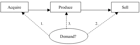
The model behind our analysis does not consider these issues separately. Given the data in Table 1, we draw correspondences between these three issues and ensure that we produce only those items we can sell and acquire only the resources we need to produce them (Figure 1). Our model and analysis exploit the
Decision Sequence:
Model:
Acquire Resources
Produce
Items Sell
Acquire Produce Sell
Figure 1: Dakota is actually faced with a sequence of three related deci-sions: How much resources to acquire, how many items to produce, and how many items to sell. The model represents these decisions as being made simultaneously, not sequentially.
structural advantages that accompany deterministic data and avoid representing potentially costly errors. In reality, the decisions occur sequentially over time.
This textbook problem is pretty straightforward. We do not need LP to solve it. However, for more compli-cated problems, an LP model is indispensable, so we describe one that considers each of the three decisions explicitly. In the following, let
yd=number of desks to produce, yt=number of tables to produce, yc=number of chairs to produce,
xl=number of board feet of lumber to acquire, xf =number of labor hours to acquire for finishing,
xc=number of labor hours to acquire for carpentry,
sd=number of desks to sell,
st=number of tables to sell, and
sc=number of chairs to sell.
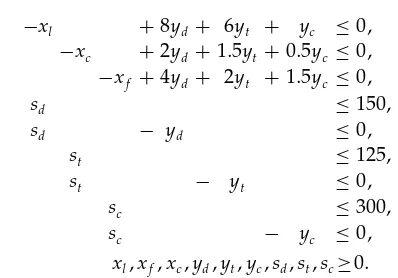
With these variables, we can formulate Dakota’s problem with the following LP:
Maximize −2xl−52xc−4xf+60sd+40st+10sc (P.0) subject to
−xl +8yd + 6yt + yc ≤0
−xc +2yd +15yt +05yc≤0
−xf +4yd + 2yt +15yc≤0
sd ≤150
sd − yd ≤0
st ≤125
st − yt ≤0
sc ≤300
sc − yc ≤0
xlxfxcydytycsdstsc≥0
raises the selling price of chairs from $10 to $11, we need only to change the corresponding coefficient in the objective function. This observation gives rise to the investigation of the solution known as SA. Know-ing that the structure of the problem does not change, we can investigate how changes in individual data elements change the optimal solution. If nothing else changes when we increase the price of chairs from $10 to $11, producing chairs becomes profitable, and the nature of the solution changes considerably. On the other hand, if the selling price of chairs remains $10, and the demand for chairs drops from 300 to 200, there would be no impact on the solution—Dakota would still not produce chairs.
Researchers use SA to study the robustness of solu-tions to LP models. That is, if they are concerned about the accuracy of the data, they perform SA to see how the solution might change if the data were dif-ferent. A change in the solution or its structure would indicate the need for further investigation. When nei-ther changes, they consider the proposed solution an appropriate guide for making the decision. The sense of security they gain from SA, however, is not well founded. Even when the solution and its structure appear to be stable, the proposed solution may be inappropriate in the face of uncertainty.
Uncertainty in LP Data
Demand for products may be uncertain, but low, most likely, and high values may be available. We will assume that the low values of demand for desks, tables, and chairs (50, 20, and 200) occur with prob-ability pl=03, the most likely values (150, 110, and 225) occur with probabilitypm=04, and the high val-ues (250, 250, and 500) will occur with probabilityph= 03. The possible demand scenarios and the corres-ponding probabilities form a distribution that we can use to describe future demand. The demand scenario presented in Table 1 is the expected value associated with the distribution in Table 2.
Analysis of the sensitivity of the solution to (P.0) indicates that our solution, “produce as many desks and tables as can be sold, but do not produce any chairs” will remain valid for any set of (nonnegative)
Item Low Value Most Likely Value High Value
Desks 50 150 250
Tables 20 110 250
Chairs 200 225 500 Probability 03 04 03
Table 2: Dakota is faced with three possible demand scenarios: Low demand values, most likely demand values, and high demand values. Each of these scenarios is modeled with specified demand for each pro-duct, and occurs with specified probabilities.
demands. Table 3 shows the optimal response to each of the individual demand scenarios.
In all cases, we produce only desks and tables, not chairs. We acquire resources to satisfy the produc-tion schedule. The producproduc-tion and resource quanti-ties in the expected-value column are the expected values of the corresponding quantities in the remain-ing columns. (This is a property of the simplicity of the example; in general, the expected value of the data does not correspond to the expected value of the solutions.) Given the stability of the structure of the solution and the relationship among the vari-ous solutions, we might think that the solution with the expected demand is an appropriate response for Dakota’s problem.
However, if Dakota produces 150 desks and 125 tables, to meet the mean demand solution, it has a 30 percent chance of producing too many desks and a 70 percent chance of producing too many tables. If it produces 150 desks and 125 tables and the
Demand
Variables Expected Value Low Most Likely High
Production quantities
Desks 150 50 150 250
Tables 125 20 110 250
Chairs 0 0 0 0
Resource quantities
Lumber (board feet) 1950 520 1860 3500 Finishing (hours) 850 240 820 1500 Carpentry (hours) 48750 130 465 875 Profit ($) 4165 1124 3982 7450
low-demand scenario occurs (50 desks and 20 chairs), Dakota’s profit will be much lower than $4,165. The costs for resources at this level are $9,835. Selling 50 desks and 20 chairs would bring in revenue of only $3,800 for a net loss of $6,035. If Dakota produced 150 desks and 125 tables and experienced the most likely demand, its net gain would be $3,565. Although not a loss, this amount is well below the projected profit of $4,165 suggested by the original LP solution.
No matter how we look at it, the analysis is flawed. If a firm bases its production on uncertain data, how great a potential error does it face? This may seem like a question SA can answer. In reality, a confusion of perspectives is at work. The LP model incorporates a kind of tunnel vision: For particular data, it tells what to do. The error analysis requires a broader view, a comparison of the manner in which the output asso-ciated with one set of data will perform if faced with something different. SA does not address this issue.
LP Models with Uncertainty
When faced with uncertainty in the demand for prod-ucts, we need a more thoughtful approach to model development. In this case, we need to capture the relationship between the times at which we will make decisions and the time at which we will know the demand. We can adapt decisions made after the demand is known to the specific demand scenario— something we cannot do for decisions made before we know the demand. To provide a proper forum for assessing the trade-offs among the various alter-natives, we need a model that captures the flexibility the decision process affords. Logically, three potential information timings are of concern (Figure 2).
1. 3. 2.
Demand?
[image:4.612.317.560.494.658.2]Acquire Produce Sell
Figure 2: When will demand be known? When demand is uncertain, it is important to know when it will be revealed to the decision maker. Will it be known before resources are acquired, between acquisition and produc-tion, or after production decisions are made?
That is, we should determine the point during the decision sequence at which we know the demand. We might have complete information about the demand before making any decisions. At the other extreme, we might not know the demand until after we acquire resources and produce items. The demand determines the actual sales quantities and consequently our rev-enues. An intermediate possibility is that we acquire resources while we are uncertain about the demand, but we set the production schedules only after we know the demand and thus have adapted to it.
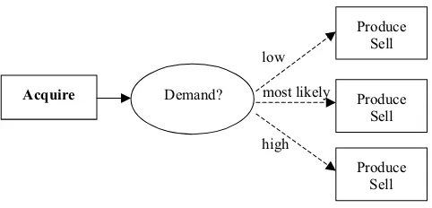
These three possibilities give rise to three different types of models. In the first case, we know demand at the start and can base decisions about acquiring resources, production, and sales on whether demand is low, most likely, or high (Figure 3).
If demand is known at the start, our decisions are not exposed to uncertainty, and we need no cross-scenario evaluation. Because all uncertainty is resolved before we make any decisions, we adapt any decision to the specific scenario realized, and the problem collapses into a collection of deterministic problems; only the origin remains uncertain. To for-mulate this problem, we need three separate sets of variables, one for each possible demand scenario (low, most likely, high). An LP model for this problem will be separable by scenario. Working from (P.0), and let-tingDdsdenote the demand for desks under scenarios (withDts andDcssimilarly defined), we obtain
Maximize
s∈lmh
−2xls−52xcs−4xfs+60sds+40sts+10scsps
(P.1)
low
most likely
high Demand
Acquire Produce Sell
Acquire Produce Sell
Acquire Produce Sell
[image:4.612.58.298.565.643.2]subject to
−xls +8yds+ 6yts + ycs ≤0 s∈lmh
−xcs +2yds+15yts +05ycs≤0 s∈lmh
−xfs+4yds+ 2yts +15ycs≤0 s∈lmh
sds ≤Dds s∈lmh
sds − yds ≤0 s∈lmh
sts ≤Dts s∈lmh
sts − yts ≤0 s∈lmh
scs ≤Dcs s∈lmh
scs − ycs ≤0 s∈lmh
xlsxfsxcsydsytsycssdsstsscs≥0 s∈lmh
As indicated, (P.1) is separable by scenario. We can consider each demand scenario separately, and we can obtain scenario-specific solutions independently. Only in calculating the objective value do we combine them. At the other extreme, we determine both acqui-sition and production before we know the demand (2 in Figure 2) (Figure 4).
Once made, the decisions about acquisition and production are fed into the demand uncertainty. Only the sales levels respond to the acquisition and pro-duction levels and the manner in which the demand uncertainty is resolved. Any LP model of this problem must capture the fact that the initial decisions must be weighed against all possible demand scenarios. To accomplish this, we use three separate sets of the sell variables, and only one set of the acquisition and pro-duction variables. As before, we work from (P.0) to develop our model. To connect Figure 4 and the LP
low
most likely
high Acquire
Produce
Sell
Sell
[image:5.612.62.293.121.255.2]Sell Demand?
Figure 4: If demand is known after acquisition and production are deter-mined, it will affect only the amount of product that is sold.
model, we use aboldfont to identify decisions made before demand is known.
Maximize
−2xl−52xc−4xf+
s∈lmh
60sds+40sts+10scsps (P.2)
subject to
−xl +8yd + 6yt + yc ≤0
−xc +2yd + 15yt+05yc ≤0
−xc+4yd + 2yt +15yc ≤0
sds ≤Dds s∈lmh
−yd sds ≤0 s∈lmh
sts ≤Dts s∈lmh
yt sts ≤0 s∈lmh
scs ≤Dcs s∈lmh
−yc scs ≤0 s∈lmh
xlxfxcydytycSdsStsScs≥0 s∈lmh
In contrast to (P.1), (P.2) is not separable by scenario. Acquisition and production, represented byx and y, are determined before demand is known and are held constant across all scenarios. The second set of con-straints models the manner in which sales depend on the combination of production and demand. The lack of separability arises because of the interaction of the two types of variables in these constraints.
Finally, in the remaining case (3 in Figure 2), we determine acquisition before we know the demand and production and sales afterward (Figure 5).
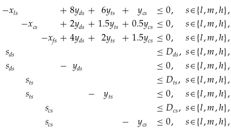
As we work from (P.0) to develop an LP model for this problem, we have a single set of acquisition vari-ables, and three sets of production and sales variables:
Maximize
−2xl−52xc−4xf+s∈lmh60sds+40sts+10scsps (P.3) subject to
−xl + 8yds + 6yts + ycs ≤ 0 s∈lmh
−xc + 2yds +15yts+ 05ycs ≤ 0 s∈lmh
−xf+ 4yds + 2yts + 15ycs ≤ 0 s∈lmh
sds ≤ Dds s∈lmh
sds−yds ≤ 0 s∈lmh
sts ≤ Dts s∈lmh
sts−yts ≤ 0 s∈lmh
scs ≤ Dcs s∈lmh
scs−ycs≤ 0 s∈lmh
low
most likely
high Acquire
Produce Sell
Produce Sell
[image:6.612.58.299.107.223.2]Produce Sell Demand?
Figure 5: If demand will be known after resources are acquired but before production levels are determined, it will affect production quantities and sales.
Similar to (P.2), (P.3) lacks separability. In general, sep-arability does not occur when the LP model includes uncertainty within the midst of the decision sequence.
Comments on Problem
Formulations and Solutions
The three LP models, (P.1) through (P.3), can be traced back to the original model, (P.0), but they differ. They represent three different models of the problem. We have little need for a model such as (P.1). Because we know the demand before making any decisions, we do not need to solve (P.1). That is, we can wait until
(P.1) Scenarios (P.0)
Mean
Variables Demand Low Most Likely High (P.2) (P.3)
Resource Quantities
Lumber 1950 520 1860 3500 1060 1,300 Finishing labor 850 240 820 500 420 540 Carpentry labor 4875 130 465 875 265 325 Demand Production Quantities Low Most Likely High
Desks 150 50 150 250 50 50 80 80 Tables 125 20 110 250 110 20 110 110
Chairs 0 0 0 0 0 200 0 0
Objective value 4165 4165 1142 1730
Table 4: Each of the problems (P.0) through (P.3) has a different optimal solution. The objective values differ as well, even when the structures of the optimal solutions are similar.
we know the demand and solve the appropriate sce-nario problem. As presented, the output of (P.1) pro-vides the optimal solution and objective values for all possible demand scenarios. For planning, this infor-mation might be helpful.
The second model, (P.2), provides a proper mech-anism for determining the expected revenues when we must determine production before we know the demand. This model accounts for the possibility that production might exceed demand. In particular, when we set production levels (which in turn determine the levels of resource acquired), we base them upon a model of the revenues that we can expect from selling them.
The third model, (P.3), separates acquisition from production. It is appropriate when we can make alter-nate production plans depending on demand that materializes from particular acquisitions. That is, it models the case in which the firm can use resources in a variety of ways to create products for which there is demand. To further appreciate the differences among the three models, we can compare their output (Table 4).
pro-duction levels suggested by (P.2) do not match any of the demand scenarios. In (P.2), production levels are set in a manner that balances the potential sunk cost of producing items that cannot be sold against the poten-tial revenue available from selling a larger number of items. This balancing act shifts the production level away from any one scenario. We cannot recognize the need for this balance with a simple SA of the tion to (P.0). More important, the structure of the solu-tion to (P.3), in which producsolu-tion decisions are delayed until after the demand is known, is distinctly differ-ent from the structures of the solutions to the other models. It is the only model that includes the produc-tion of chairs in the optimal soluproduc-tion and then only in the low-demand scenario. The interpretation of this solution is clear. Although chairs on their own are not profitable, their production in some cases is advanta-geous. The solution to (P.3) includes acquisition of a larger amount of resource than the solution to (P.2). When the demand is high enough, all of this resource goes toward the production of desks and chairs (the profitable items). However, when the demand is low, production of chairs offers the firm an opportunity to recoup much of the cost of the resources acquired. The chairs provide the firm with a fallback position that permits an aggressive resource acquisition plan. Again, we cannot realize the advantages of this adap-tation with a simple SA of the solution to (P.0).
The various objective values differ as well. It is well known that solving an LP in which random variables in the right-hand sides of the constraints are replaced by their expected values yields an opti-mistic objective value, as indicated in (P.0) compared to the rest. Indeed, in this case, (P.0) is as optimistic as (P.1), in which the decision maker knows all informa-tion before making any decisions (although this need not be the case in general)! That the objective value for (P.3) exceeds that of (P.2) is no surprise; delay-ing decisions until one has information usually brdelay-ings economic advantages. To determine the appropriate model, one must identify the point at which informa-tion about demand will be available.
Alternate Objective Functions
Our LP models have the objective of maximizing expected profit. There are many valid criticisms of
Profit Generated
Demand Probability Alternative 1 Alternative 2 Alternative 3
Low 0.3 0 −100 −300 Most likely 0.4 0 0 −300
High 0.3 0 −100 700
Table 5: The three alternatives yield different profits for each demand sce-nario. The expected value of the profits associated with all three alterna-tives is zero.
this choice of objective function. Because the expected value is a linear functional, gains and losses can can-cel each other out. That is, suppose that we have three alternatives that yield profit distributions as a func-tion of demand (Table 5).
Given the objective of maximizing expected profit, we would not distinguish between these three alter-natives. This lack of distinction is inconsistent with most people’s attitudes toward risk—most people have a clear preference among these three alterna-tives. The economist addresses this problem through utility theory, using a utility function that encapsu-lates the trade-off between expected profit and risk to guide the decision-making process. In general, optimization of expected utility requires a nonlinear objective function, although piecewise linear approx-imations can often be developed. In addition to the changes in the constraints, uncertainty may also result in a change in the objective function.
Discussion
at which decisions are made and the times at which we have certain data.
In most cases, the output of SA is misleading when used to assess the impact of uncertainty. SA is most appropriate when the basic structure of the model is not altered by the presence of uncertainty—for exam-ple, when all uncertainties will be resolved before any decisions are made. When the decisions are to be made, a deterministic model will be appropriate, but as long as the data is uncertain, we do not know whichdeterministic model will be appropriate. In this situation, SA can help us to appreciate the impact of uncertainty. In all other cases, we cannot count on it to do so.
SA fails as a tool for gauging the impact of uncer-tainty because it cannot capture the possibility of a response to information. When we obtain infor-mation during a decision sequence, we have the opportunity to adapt to it. Whether the adaptation is imposed, as when sales are constrained by demand, or advantageous, as when production decisions can be delayed until after demand is known, adaptation causes changes in the LP model. The constraint matrix changes considerably, affecting both the number of constraints and the number of variables. Because SA depends on an enduring structure in the LP model, it is not an appropriate tool for identifying the impact of uncertainty in these cases.
Conclusion
Under uncertainty, we cannot predict the conditions we will face tomorrow. A decision made today affects what we can do tomorrow. Similarly, what we ulti-mately decide tomorrow will depend on what we have learned today. Today’s decision should be bal-anced against the conditions that we might face so that we can be reasonably confident about the posi-tion that we will be in tomorrow. When a model is based on the presumption of deterministic data, learning is absent in both the model and its output. SA based on the output of such a model will not reflect an ability to adapt to information that becomes available within a sequential decision process. It does not perform the balancing act required for decision making under uncertainty.
Acknowledgment
We gratefully acknowledge the Centre for Advanced Study at the Norwegian Academy of Science and Letters, whose support during the 2000–2001 academic year made this work possible.
Reference