Managing multiple spaces

Managing Multiple Spaces

Lancaster University [email protected], [email protected]

Boriana Koleva, Tom Rodden Nottingham University [email protected], [email protected] Henk Muller, Cliff Randell

Bristol University [email protected], [email protected]

Anthony Steed

University College London [email protected]

1.

Setting the scene

This paper is about our experiences of space in the Equator project (www.equator.ac.uk), in particular, the way in which multiple spaces, both virtual and physical, can co-exist. By this we mean that people and objects may have locations in and relationships to both physical space and one or more virtual spaces, and that these different spaces together interact to give an overall system behaviour and user experience. The concepts we develop in this chapter are driven partly by practical experience, and partly by previous theoretical work such as the models and taxonomies of spatial context in (Dix et al., 2000), the models for mixed reality boundaries (Koleva et al., 1999) and capturing human spatial understanding exposed in sources such maps, myths and mathematics (Dix, 2000). We are also building on established work on informal reasoning about space from the AI and GIS communities (Grigni et al, 1995; Papadias et al., 1996) similar to Allen’s well known temporal relations (Allen, 1991).

We start by looking at some of the practical experiences in a number of Equator ‘experience’ projects and how these have each required several kinds of interacting spaces: real and virtual. We then use this as a means to look more abstractly at different kinds of space and the way these overlap and relate to one another. In order to examine some aspects in greater detail we will use two artificial scenarios which each highlight specific problems and issues. Finally, we will discuss how this is contributing to ongoing work including the construction of an Equator ‘space infrastructure’.

2.

Spaces we have known

Equator is a large multi-site multi-disciplinary project focused on the integration of digital and physical interaction. One of the key methods used in Equator are ‘experience projects’. These experiences are focused around the creation of a particular event or outcome, which allow the integration of practical and theoretical work of many kinds. As the focus of Equator as a whole is the confluence of physical and digital life, unsurprisingly the nature of space has been important in many of these sub-projects. We will discuss four of these here: City, CityWide, the Drift Table and Ambient Wood. In each we will see multiple physical and virtual spaces interacting.

2.1 City

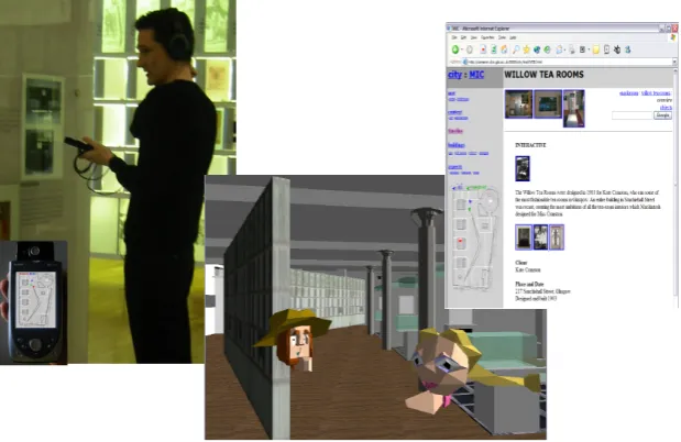
mackintosh room tracked by ultrasound beacons and has a handheld PDA. The VR visitor navigates a desktop VR model of the Mackintosh Room and can see the various exhibits within the rendered world. The web visitor navigates between web pages organised by sections of the Mackintosh room and can see exhibits on the web pages. All three visitors can talk to one another using a microphone and ear-piece and so can discuss what they see. The visitors can also see one another on a map view: shown on the PDA for the physical visitor, and on screen for the VR and web visitors. Also the VR visitor can see avatars representing the physical and web visitors within the VR space.

As well as the physical space of the museum there is a digital reproduction of it for the VR users and a map view used by all. In this virtual map, the VR visitor has a precisely known ‘position’ within the virtual room. In contrast the web visitor doesn't have an explicitly defined position because they can't actively move themselves around the map. Their position is inferred from their web page browsing: they are implicitly positioned on the map in front of the objects represented in the web pages they are reading. The real visitors of course have a precise position known to them. However, this physical position is sensed using ultrasound, which has limited resolution, varying degrees of accuracy and even coverage black spots within the physical space. Furthermore the ultrasound date then has to be mapped to a physical location lading to further issues.

In fact a detailed analysis revealed seven spaces that impinge directly upon the user not to mention various coordinate spaces used internally within the software (Steed et al., 2004).

Figure 1. Views of the physical, VR and web visitors

2.2 CityWide

'Can You See Me Now?' was staged in Sheffield in December 2001, in Rotterdam in February 2003 and in Oldenberg in July 2003 and attracted over 1500 online players. It was awarded the 2003 Prix Ars Electronica Golden Nica award for Interactive Art (for the Rotterdam performance) and was nominated for a BAFTA in Interactive Entertainment in 2002 (for the initial Sheffield performance).

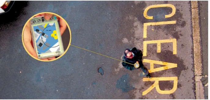
In ‘Can You See Me Now?’ the virtual and physical spaces are overlaid as if there were an invisible ghostly realm behind the surface of buildings and streets. Again varying degrees of accuracy of the GPS sensors used to track the physical participants mean that the measured locations available to the virtual participants may not represent truly the actual physical locations. In particular, GPS accuracy was particularly poor in the ‘shadow’ of buildings as the performances of ‘Can You See Me Now?’ were always staged in densely packed city spaces where it is hard to get a good GPS fix without multi-path reflections.

Figure 2. Can You See Me Now? runner carrying PDA display

2.3 Drift Table

Figure 3. The Drift Table moves across a photographic model of the UK countryside

Although conceptually and physically very simple the Drift Table both hides technical complexity and elicited rich interactions. Within the form factor of the coffee table is a PC, screen and disk array large enough to store over a terrabyte of map data. The table also has weight sensors that are used to determine the direction and speed of travel. At a maximum virtual speed of only a few tens of miles an hour, if the owner of the Drift Table wanted to ‘go somewhere’ specific he had to place heavy objects on one side of the table and then leave it for several hours before making adjustments.

2.4 Ambient Wood

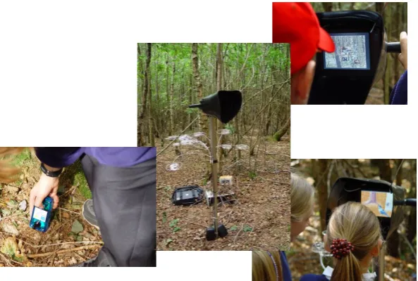
Finally, in Ambient Wood, school children wander around a wood in Sussex on a ‘digitally enhanced field trip’. The aim of the experience is to reveal using digital augmentation the features of the natural environment that would otherwise be invisible (Price et al. 2003). The children work in pairs and use a humidity and light sensor as they explore the wood. The location of their readings are recorded so that they can be shown later collected together on a map of the wood. As they move through the wood there are zones determined by radio 'pingers'. When the children enter a zone sounds or other events are triggered. For example, in one zone they can listen to the vastly amplified sound of a butterfly sipping nectar.

Deep within the wood the children find a somewhat enigmatic device, the periscope. Atop of a branching metal structure is a cowled screen. As the screen is rotated it shows the wood as it would be under different conditions, for example, if a new organism were introduced. The periscope acts like a magic viewport that overlays a virtual view of the wood over the real one. The sense of connection was so strong that children would stand the other side of the periscope expecting to be visible in the virtual view.

Figure 4. Activity in the Ambient Wood: moisture reading and periscope

3.

Understanding space

As we have seen each of the experience projects has involved multiple spaces some physical some virtual. In this section we will examine at a more abstract level the kinds of spaces involved. First we will look at three levels of virtuality from physical space, through the measured coordinates of real space and objects to virtual spaces. We will then look at three kinds of location systems used for measured space which also correspond to ways in which we envisage real space. Finally in this section we will look at the way overlapping or adjoining spaces map onto one another and how people and computers can manage this intersection.

3.1 Three kinds of virtuality

Augmented and mixed reality clearly involves physical space and virtual space. However there are, in fact, three types of space to consider:

• real space – the locations and activities of actual objects and people in physical space • measured space – the representation of that space in the computer and the representation

of locations of objects and people from sensor data, etc.

• virtual space – electronic spaces created to be portrayed to users, but not necessarily representing explicitly the real world

measured space

virtual space real

space

cartography & calibration

subject matter

projection

extent of target

point of projection location

sensing

triggers and anchors

identification

Figure 5. Three kinds of space and relations between them

These three types of space are related in different ways. In each case there is a static relationship between the spaces themselves and a more dynamic relationship about the actual sensing of physical things, the events and behaviours triggered by them in the virtual world and the projection of virtual world back into the physical.

3.1.1 real – measured

In order for a measured space to be meaningful it must in some way correspond to aspects of the physical space. This will involve a process of mapping the fixed aspects of the real space using some cartographic measurement of points and their relations, either against a global system (e.g. GPS) or relative to one another (e.g. theodolite or simple tape measure).

This may be a fixed once-and-for-all process but may involve a more dynamic recalibration if the space is not fixed. For example, the variation of air pressure due to weather systems means that the ground can rise or fall by small but measurable amounts. At a slower time scale plate tectonics means that the ocean floor under, for example, the Atlantic is slowly splitting. Measures of longitude therefore change in the order of centimetres from year to year. If location sensing were being done in Iceland then this would even affect relative locations of cities and buildings. Later we will discuss coordinate systems on board moving trains which change even more rapidly.

Given a measured space we then obtain the location of objects within that space using some form of sensing. This sensing may vary in accuracy. For example, in ‘Can You See Me Now?’ the GPS sensors were more accurate in the open and less accurate when behind the shadow of buildings. This difference is not insignificant and accuracy can vary from a few metres to tens of metres. Furthermore there are areas such as within buildings where the GPS signal disappears completely. In the Mackintosh room there were similar problems as the ultrasound transmitters were placed on top of exhibits (so that they were visually unobtrusive), but this meant that booth-like areas in the room were black-spots where the reading of location was effectively meaningless. Note that here the signal was not just inaccurate (a radius within which the real value lies) but misleading.

one not always a realised one. We know that the interior of the car has a physical location in space and as such has constraints of physicality in its coordinate system and objects. However, we may have no idea exactly where in physical space it is!

This relationship to real space actually shows up in the limits on the interrelationship of measured space as in some way the real space is as virtual to the electronic space as the electronic is to the physical.

3.1.2 measured – virtual

In the case where the virtual space corresponds to a model of the physical one then there may be a close mapping between measured and virtual spaces. For example, in Ambient Wood location of a moisture or light reading is first derived in a measured space of GPS coordinates. This is then related to the coordinates of a map of the wood on which the readings are later plotted. Similarly in the Mackintosh room ultrasound location is measured to give a coordinates which are then mapped onto the 2D map and 3D virtual room.

We have labelled this ‘identification’ in figure 5 as this is often a (relatively) straightforward identification of measured coordinates to their corresponding virtual ones. Sometimes the virtual space may not represent the same space as the physical one, but there may still be an identification between the virtual and measured/real: for example, we may make locations in real space map onto locations in an information space so that we can walk around the real space and navigate the virtual.

In the case where there is not a direct mapping between real and virtual this identification between measured and virtual may also be relative rather than absolute. That is a direction of movement in the measured space may give rise to some corresponding movement in the virtual. There is an element of this in the use of weights in the Drift Table although one could imagine having more complex explorations of non-planar spaces.

Whether or not there is a relationship between the measured space and virtual, particular locations or events in the measured space may trigger actions in the virtual space The many tourist and museum information systems are examples of this as is the Stick-e Note infrastructure for location and context-sensitive interaction (Pascoe, 1997). We have also an example of this in the way proximity to a pinger in the Ambient Wood triggers an information source.

Note that as these are triggering electronic world events they will normally (always) be triggered from representations of the objects and space in the measured spaces rather than directly by the physical space. Arguably something like triggering by physical contact or capacitance would be a counter-example. However, even then the event cannot be used to trigger virtual actions unless it is sensed. In this example, the sensing is effectively a relative one “these two objects are near each other” and we’ll return to issues of relative location later.

3.1.3 virtual – real

The virtual world may in some way represent or be about a particular real space. For example, a web page about London, or a virtual model of the Eiffel Tower. Several of the spaces we have seen are like this: the virtual Mackintosh room, the virtual model of the city streets in CityWide, the aerial photographs of the UK in the Drift Table.

The Drift Table is interesting in that it is partly corresponding to the real world: if reset it centres itself above the actual location of the table. However, the height and movement of the table means that is more often a view of ‘somewhere else’.

Virtual spaces are made available in the real world by being projected, usually visually but also audibly or even by other means such as tactile or haptic devices or even smell (Burdea, G.C. & Coiffet, P. 2003). When the virtual world is made manifest it must be at some particular point in the real world. This has various aspects:

• point of projection – The device that embodies the projection is actually in the real space (on a screen, in virtual reality goggles, in the the Ambient Wood periscope, on the Drift Table porthole, on a runner’s PDA in ‘Can You See Me Now?’)

• range of detection – There will be a set of locations in the real world where the projection can be seen (or heard, smelt etc.)

• extent of target – The projection appears to occupy some part of real space, usually ‘behind’ the projection surface for visual projections. For example, in a video wall, the space being projected would appear to be ‘the other side’ of the screen – that is occupying actual space (albeit through a wall!) Again in the Drift Table it appears as though the places in the photographs are somewhere far below and the room floating above. Although the extent is usually ‘behind’ the point of projection, when viewing a hologram the extent is actually in front of the holographic plate and in an augmented or immersive virtual reality using stereo goggles the extent of projection may appear to be everywhere.

Note that video and audio office shares, CCT video or web cams have similar aspects. When you look at a picture on a cinema screen there is a sense in which the image purports to occupy space behind the screen.

3.1.4 the interaction cycle

Note that there is a cycle of interaction here different but reminiscent of the Model–View–Controller (MVC) model for graphical user interfaces (Krasner & Pope, 1988). In fact if one thinks of the location of a puck or mouse being sensed and mapped onto the virtual screen space it seems uncannily close. However, there is a major difference in that (except for specialised devices such as digitising tablets), the physical location of mouse or puck is only important insofar as it controls the virtual space of desktop and screen cursor. In contrast, in mixed and augmented reality experiences, the locations of sensed objects typically have meaning in the real world as well as the virtual.

However, the MVC parallel can teach us something about this mixed reality interaction cycle. One of the tensions of the MVC model is the coupling between the Controller and View. In a simple pipeline interaction model the input (mouse actions or keystrokes) would be processed by the Controller, converted into abstract actions on the Model, leading to changes in the Model state, which are then rendered by the View on the screen. This works for actions such as pressing control-X to cut an object to the clipboard, but not for true graphical actions such as clicking a mouse over an object to select it. To interpret the latter the Controller needs to know what is where on the screen, and so has to ‘ask’ the View what is rendered at a particular screen location.

matters is that the location of the torch beam is correctly registered relative to the projected virtual space.

3.2 Three kinds of location system

So, when we talked about the measured and virtual spaces as having their own coordinate system, we really mean something more like location system as not all are based on Cartesian coordinates as such. Even physical space has different characteristics depending on perspective: "in this room", as opposed to "near Aunt Mo" or "at 37.32E, 12.56N". Notice also how this location information is of very different kinds:

• coordinates – This is where location is in some sort of explicit dimensional representation, not necessarily orthogonal and not necessarily Euclidean (e.g. polar, spherical, UK Ordinance Survey (OS) grid). Note that these coordinate systems will typically only have validity over a finite space (the OS grid is meaningless over North America) and have an even smaller space over which they are expected to have values. For example, a coordinate system based on x,y,z locations in the Mackintosh room would have validity over central Glasgow, but would only be expected to be used within the room. In the case of the Mackintosh room the coordinates are never needed beyond the room, but of there were also sensors in the corridors outside, then the link between the two would be important.

• zonal – This is where objects are located within some area. For example the Pepys system used IR-based Active Badges simply to record presence in a room (Newman et al., 1991). Mobile communications typically give some level of zonal information ‘for free’: a mobile phone can use the current cell to give tourist information or even ‘push’ advertising and in several systems, notably the early work on the ‘GUIDE’ tourist system, the current WaveLan base-station is used as a proxy for location (Cheverst et al., 2000).. The simplest form of zonal space is a single proximity sensor such as the pinger in Ambient Wood. • relational – This is where objects report some form of relative location information: device

A is close to device B, or device A is about 3 metres north-east of device B. This leads to a space which can be regarded as a graph of all the possible sensors/devices with knowledge of some arcs (approximate distance, possibly direction) and sometimes knowledge between arcs (angle between devices). It is interesting to note that most traditional cartography starts with precisely this information. The simplest form of relational information is also simple proximity, for example, detection of which Bluetooth devices are in range..

Furthermore, measured spaces differ in both accuracy and extent. For example, the ultrasound location in the Mack room only has meaning within the room and even then has voids in information booths that create an ultrasound shadow. In fact, apparently unambiguous cartographic systems such as the OS Grid have limitations as the earth beneath our feet is constantly shifting due to continental drift and even atmospheric conditions.

Note too that these location systems relate principally to the way in which objects are represented within the space. So that even in a zonal space, the zones may have known physical extent within some coordinate system but the objects only known to the granularity of the zone. Also even where detailed coordinates are known they are often converted in zones which represent conceptual regions, for example, around exhibits in the Mackintosh room.

with location this information may be Cartesian (e.g. compass direction), zonal (e.g. facing the window) or relational (e.g. two people facing each other).

3.3 Three kinds of relationships

As we saw in the examples earlier, it is not that we have a single measured, real and virtual space, but typically several of each. These multiple spaces are related in various ways. Again these seem to be of three kinds:

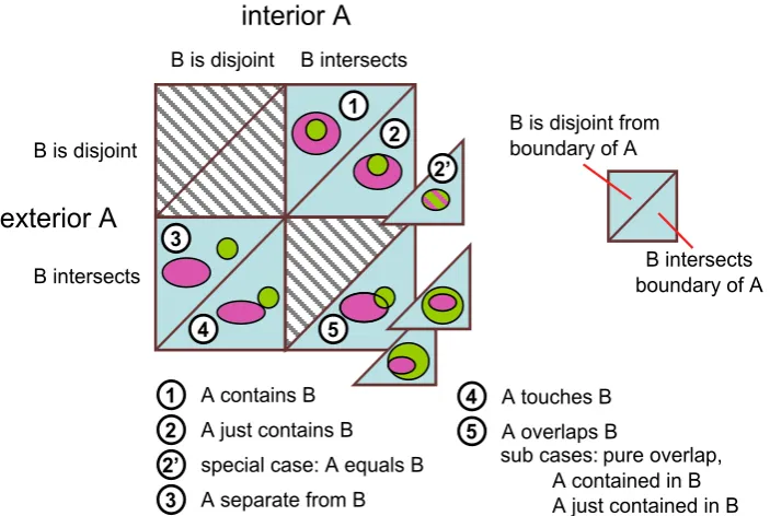
• topological – There are a standard set of qualitative relations between regions of space: separate, overlaps, touches, contains etc. (see figure 6) and also relations between lines and regions that are used for qualitative reasoning in AI. For example, Grigni et al. (1995) give inference rules for proofs about this type of spatial relation and Papadias et al. (1996) uses a richer set that takes into account directions (e.g. to the east of) and hierarchical relations between spaces in spatial databases. There is a similar set of temporal relationships (before, overlaps end, etc.) defined by Allen (1991).

These topological relations are usually applied to sub-regions of a universal space. Where we are dealing with spaces in the real worked, this is the case (at least in principle, although measuring may be difficult), but most of the measured and virtual spaces we are dealing with are effectively independent until we define the relationship between them. The second two kinds of relationship are about this.

• boundary – We may have two locational systems that have no substantive overlap, but where there are boundaries that can be traversed. For example, we may have ultrasound sensing in two different rooms and objects may pass from one to the other. As we have already seen when discussing projection, these boundaries can also occur between the real and physical. Koliva et al. (1999) discuss in detail the properties of these mixed reality boundaries including the permeability of the boundaries: whether light, sound, objects can traverse them.

interior A B is disjoint B intersects

B is disjoint

B intersects exterior A

B is disjoint from boundary of A

B intersects boundary of A 1

2

3

4 5

2’

1 A contains B 2 A just contains B 2’ special case: A equals B

3 A separate from B

4 A touches B 5 A overlaps B

sub cases: pure overlap, A contained in B A just contained in B

Figure 6. Qualitative relations between regions of space

For the topological relationships the issue of the extent of the 'normal' area of the space becomes important. We are not talking about the coordinate system intersecting but the natural regions that the spaces represent. That is we have two very distinct ontological categories:

• space as extent within another (perhaps not measured) • space as potential to measure locations

Topological and existence of boundaries relates primarily to the former. Mapping and mapping at boundaries is largely about the latter.

Following the mathematician's habit of always looking for structure-substructure relationships it is clear that there are some here. In coordinate spaces virtually any region may (with some transformation of coordinates) be regarded as a subspace. Similarly the local coordinate space of an individual device in the 'relational' system may be regarded as either a zonal or coordinate space in its own right.

There may be some advantage in being clear about this as it stops angst about whether the 'space' is one thing or another. We just say both!

Operationally, in any application we need to decide what we represent as spaces (although even then things may be used in different ways at different times), and also what are 'heavy-weight' spaces with permanent representations and what are light-weight ones used when appropriate.

The subspace relationship is also complicated by various factors including the dynamic relationship between spaces and location systems.

3.4 Managing multiple spaces

ultrasound location sensing would not be lost. This gave the remote participants a more accurate view of the physical participant’s location (albeit being portrayed just outside the booth). As we saw the user of the Drift Table brought maps and atlases into the experience – choosing voluntarily to add yet more spaces.

Computationally things are more difficult!

In mathematics differential geometry deals with spaces that are curved or broken in ways such that no single coordinate system can cover them. Instead a patchwork of overlapping coordinate systems are used with mappings in the areas of overlap. Depending on the type of mathematics being done the mappings are required to have different kinds of properties. for example, to deal with general relativity the mappings are usually required to be ‘smooth’ – infinitely differentiable.

A more mundane example of this can be seen in a world atlas. The earth is roughly spherical (flattened slightly at the poles) but atlas pages are flat. You can imagine wallpapering a spherical globe with the separate maps. At the overlaps there is a mapping between the local coordinate systems of the individual maps’ Cartesian coordinates even though there is no overall ‘flat’ coordinate system. Note too that the earth is no a series of flat faces, each page of an atlas is a slight morphing of the actual earth’s surface. For a small area like a building or town, the approximation form this flattening is insignificant for all but the most accurate measurements, but at the scale of countries the edges tend to become distorted. Different map projections make choices about which areas are most ‘true’ and which more distorted. For example, the Phillips projection is most ‘true’ (in the sense of ‘flat’) at the latitude of Southern Europe whilst the equator is very stretched North South and the poles squashed. In contrast the more common Mercator projection manages to be true (in the sense of flat) everywhere (called a conformable mapping), but at the expense of distorting the relative sizes of countries and not being able to cover the polar regions.

Similar techniques are used in VR systems, often called locale-based models (Barrus et al., 1996). Two rooms may have separate VR models which are linked at the doorway by a local mapping between the coordinate systems. Given these spaces are constructed and Cartesian the mappings are usually well behaved. This may be either a simple scaling and translation of origin or at worst an affine transformation. This boundary mapping means there does not have to be a single super model and so makes the virtual world more computationally tractable and easier to manage. The boundary mapping is then used when objects move between the worlds, or to trace light rays so that one space can be seen from another.

Note however that in all these case the partial spaces are Cartesian and also that the mapping is largely fixed. Unfortunately, neither are necessarily true in the digitally enhanced environments we are considering.

4.

Scenarios

train) moves relative another coordinate system (the track and stations) and is not even of constant shape (the train bends).

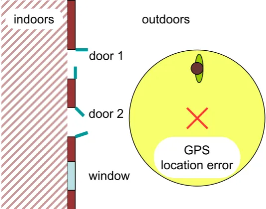
4.1 Twin doors

This scenario is focused on issues that arose due to uncertainty in location sensing when you move between two spaces that are measured using separate technologies. Imagine a building with two doors, as shown in Figure 7. People walk in and out of the building, and are tracked using two types of tracking devices. For outside tracking GPS is used with an accuracy of around 3m, and for inside tracking a more accurate system is used, for example an ultrasonic positioning system with an accuracy of 10cm.

In order to describe this scenario properly, we need at least two spaces. There is the Outside of the building, which is a space that is measured using spherical coordinates obtained from a GPS sensor. We will assume that locally these coordinates are Euclidian. Secondly, there is the Inside of the building, which is at least one space, but there may be one space for each room. The inside-space is described using Cartesian coordinates.

In addition there are two conceptual spaces: the personal spaces of the people who are walking through the doors, and the physical space that these people live in.

GPS location error indoors

door 1

door 2

window

outdoors

Figure 7. Twin doors – physical situation

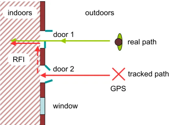
Scenario – sudden shifts in positions and walking through walls

is possible that the GPS location was right and the ultrasonics system was disturbed by some noise.

indoors

door 1

door 2

window

outdoors

tracked path real path

RFI

GPS

Figure 8. Twin doors – wrong door?

The most important issue to resolve here is how to present this discontinuity outside the location infrastructure. Devices that Alison carry around, devices in the building, or people may need Alison’s position. In addition to the position, the path that Alison walked may be requested.

An obvious question is whether the discontinuity should be smoothed out. For example, from GPS and ultrasonics accuracy the system can deduce that the ultrasonics is probably right and the GPS is probably wrong, and the system can hence retroactively alter its representation of the path that Alison walked to gradually go from the red cross to door 1. A problem with smoothing it out retroactively is that applications that request the path twice in a row may get two entirely different answers. On the other hand the position can be smoothed out form door 2 to it correct position, but this knowingly records incorrect positions. This leaves us with the option of not correcting the discontinuity, and leaving the problem to be solved by some other part of the system.

The ‘right’ answer on how to represent the discontinuity depends on the context, who asks the question, etc. It seems fairly sensible that if we wanted to ask the question the next day “where did Alison start off” then we should use the correction using the ultrasonic location sensing and work out it was opposite door 1. However, if we were looking at an accident enquiry it may be important what other people saw at the time, and to record uncorrected information.

Variant scenarios

What if Alison and Brian have bluetooth devices which sense one another's presence (relational space) and report this to the other spaces. How do we deal with conflicting information? If we choose to represent things as a single model of “how things are” in measured space (pretty much how our own brains work), then we are forced to make decisions early between conflicting and partial location information. Alternatively we may simply hold all the evidence (measurements by different systems at different times) and put off dealing with conflicts until decisions are really required. However, this is likely to be both computationally intractable and lead to its own paradoxes.

4.2 On the train

We now consider a scenario designed to expose issues of moving spaces. Consider a train that has various forms of location sensing within it. This will clearly make a 'space' of locations within the train, but this space itself both moves and bends within the stationary space of track, buildings etc. (Figure 9).

There are four obvious spaces that need to be represented. First, there is the Outside Space. This space is is fixed and mapped to Ordinance Survey grid or perhaps GPS coordinates. Second there is a Train Space. This space is conceptually linear (in that it consists of a sequence of carriages), but not necessarily straight, as the train may move around a bend in the track. The granularity that is required is low – “I want to get from seat 3F in carriage G to the buffet car”. Within a carriage we find the third space, the Carriage Space, which can be represented with a Cartesian system. Finally, there are Seat Spaces requiring fine granularity. For example, to place a paper 'reserved' ticket in the slot in the seat back requires millimetre accuracy.

(c) carriage space

(d) seat space (a) world’s

stationary

space _{(b) train}

space

A

B

C

D

E

F

G

H

Figure 9. Train spaces

Scenario – Getting onto the train

Alison is on the train and Brian is on the platform. As the train starts off Brian keeps pace and starts to say something to Alison through the window. Alison cannot hear through window and the noise of the engine, but can see his lips moving. He runs along beside the train until it gets too fast and he is left behind. It is one of those old fashioned trains with open steps and as the open doorway passes he swings himself up into the train.

In this scenario Alison’s location is measured relative to the carriage and seat spaces and she is not 'moving' relative to them. The carriage space is also static in the train space, but the train space is moving relative to the world space. Brian’s location, as measured in the world-space using GPS is changing. Brian and Alison are staying near to each other because the change in Brian’s location, matches the way that the train space is moving relative to the world space. There are two boundaries between the spaces that are worth discussing. The train window is permeable to vision, but not sound or movement. The window is moves relative to the stationary space, but is stationary relative to the carriage space. The doorway is similar to the train window, but it is permeable to movement. By stepping through this door, Brian stops being in motion relative to the world space, and becomes present, stationary, in the moving train space.

Scenario – Moving through the train

Brian is walking quickly down the train to find Alison. Someone's feet are sticking slightly into the gangway and he half trips over them.

“Oops”, he says and he turns

“Sorry”, says the person sitting at the seat

Then he recognises the person as Clare, another work colleague. After a polite chat with Clare, Brian continues down the train. As he passes the seat of Dave, he meets the ticket collector. Brian does not have a ticket, and he searches for some cash in his pockets to buy a ticket. All this time they stand at Dave's seat.

In this scenario, Brian is moving primarily in the train and carriage spaces. He is not concerned what is happening on the seat space. Only when he trips, his attention shifts from the carriage space to the seat space. This shift in attention was not planned or intentional, and it will be difficult for a system to tell that this shift has happened. If we want to detect that Brian has ‘met’ Clare, then the best we can do is to use the time of residence within a zone as a measure of focus. However, if time in proximity were used as a heuristic for entering the seat space, Brain would have been regarded computationally as in Dave's seat space when he was buying a ticket, and perhaps a meeting with Dave was logged incorrectly.

Scenario – leaving the train

While the ticket collector is issuing the ticket, the train stops at a station and then starts again. As they finish, Brian looks out through the train only to see Alison slowly moving past the window. She is standing on the platform looking at the information board while the train moves off to the next station. Brian's words are unrecorded.

boundary does not imply there is contact, the people on either side need to focus in order to establish contact.

5.

Future work – from theory to infrastructure

The experience projects described earlier in this chapter were built using a variety of existing and specially constructed mechanisms. Building interactive experiences and applications that exploit space and location requires both low-level underlying infrastructure for linking sensors and managing spatial information and also high-level tools to aid content developers to produce spatially triggered information.

Ongoing work in Equator is addressing several of these issues. At the level of location sensing the deployment of indoor ultrasonic is being made more easy by using automatic calibration instead of requiring accurate measurement of transmitter positions (Duff & Muller, 2003). Also signals from public WiFi access points are being used to give location information in town centres without the need for expensive GPS receivers. At the tools level both designer-controlled methods using ‘colouring’ of maps and also by-example learning are being used to create semantic zones within continuous coordinate spaces. Finally at the infrastructure level a single spatial infrastructure is currently under construction.

For information about this ongoing work on space see:

http://www.hcibook.com/alan/papers/space-chapter-2004/

6.

Summary

In brief, we have seen how experiences with digitally enhanced environments reveal multiple interacting spaces. We distinguished physical, measured and virtual spaces and saw how each can be of several kinds and differ in accuracy and extent. People deal remarkable well with complex special relationships, but it is harder for mere computers! In order to understand the mappings between these complex spaces we have been using scenarios to explore different types of space, complementing our more practical observations.

References

Allen, J.E. 1991, 'Planning as Temporal Reasoning', in Proc., 2nd Principles of Knowledge Representation and Reasoning, Morgan Kaufmann.

Barrus, J. W., Waters, R. C., & Anderson, D. B. 1996. Locales: supporting large multiuser virtual environments. IEEE Computer Graphics and Applications, 16(6):50–57.

Brown, B., McColl, I., Chalmers, M., Galani, A., Randell, C. and Steed, A. 2003, ‘Lessons from the Lighthouse: Collaboration in a Shared Mixed Reality System’. In Proc. of the CHI 2003 Conference on Human Factors in Computing Systems, ACM Press, pp. 577–584.

Burdea, G.C. & Coiffet, P. 2003, Virtual Reality Technology, 2nd Edition, Wiley-Interscience. Cheverst, K., Davies, N., Mitchell, K., Friday, A. & Efstratiou, C. 2000. ‘Developing a

Context-aware Electronic Tourist Guide: Some Issues and Experiences’. In Proceedings of CHI 2000, ACM Press, pp. 17–24.

Dix, A. 2000, 'Welsh Mathematician walks in Cyberspace (the cartography of cyberspace)', in Proc. of the Third International Conf. on Collaborative Virtual Environments -CVE2000, ACM Press, pp. 3–7.

Duff, P. & Muller, H. 2003, ‘Autocalibration Algorithm for Ultrasonic Location Systems’. In: Proceedings of the Seventh IEEE International Symposium on Wearable Computers, IEEE Computer Society, pp. 62–68.

Flintham, M., Anastasi, R., Benford, S., Hemmings, T., Crabtree, A., Greenhalgh, C., Rodden, T., Tandavanitj, N., Adams, M. & Row-Farr, J. 2003, ‘Where on-line meets on-the-streets: experiences with mobile mixed reality games’. In CHI 2003 Conference on Human Factors in Computing Systems, ACM Press Florida, 5-10 April 2003.

Gaver, W., Bowers, J., Boucher, A., Gellerson, H., Pennington, S., Schmidt, A., Steed, A., Villars, N. & Walker, B. 2004, ‘The drift table: designing for ludic engagement’, In Design expo case studies: Extended abstracts of the 2004 conference on Human factors and computing systems table of contents, CHI 2004, Vienna, Austria. pp. 885–900

Ghali, A., Boumi, S., Benford, S., Green, J. & Pridmore, T. 2003, ‘Visually Tracked Flashlights as Interaction Devices’, in Proceedings of Interact 2003, Zurich, Switzerland, IFIP.

Grigni, M., Papadias, D. & Papadimitriou, C. 1995, 'Topological Inference', in Proceedings of the International Joint Conference of Artificial Intelligence (IJCAI), Montreal, Canada, AAAI Press.

Koleva, B., Benford, S. & Greenhalgh, C. 1999, 'The Properties of Mixed Reality Boundaries', in Proceedings of ECSCW’99.

Krasner, G., & Pope, S. 1988. ‘A cookbook for using the model-view-controller user interface paradigm in Smalltalk-80’. JOOP, 1(3).

Newman, W., Eldridge, M. & Lamming, M. 1991. ‘Pepys: Generating Autobiographies by Automatic Tracking. In Proceedings of the second European conference on computer supported cooperative work – ECSCW '91, 25-27 September 1991, Kluwer.Academic Publishers, Amsterdam. pp 175–188.

Papadias, D., Egenhofer, M. & Sharma, J. 1996, 'Hierarchical Reasoning about Direction Relations', in Proceedings of the 4th ACM-GIS, ACM Press.

Pascoe, J. 1997. ‘The stick-e note architecture: extending the interface beyond the user’. In Proceedings of the 2nd international conference on Intelligent user interfaces, ACM Press, pp. 261–264

Price, S., Rogers, Y., Stanton, D. & Smith, H. 2003, ‘A new conceptual framework for CSCL: supporting diverse forms of reflection through multiple interactions’. In Wasson, B., Ludvigsen, S. & Hoppe, U. (eds), Designing for Change in Networked Learning Environments. Proceedings of the International Conference on Computer Supported Collaborative Learning 2003.