A Modified Interactive Stability Algorithm for Solving Multi Objective NLP Problems with Fuzzy Parameters in Its Objective Functions

(1)

http://dx.doi.org/10.4236/ajor.2016.61002

How to cite this paper: El-Hady Kassem, M.A., Tarabia, A.M.K. and El-Badry, N.M. (2016) A Modified Interactive Stability Algorithm for Solving Multi-Objective NLP Problems with Fuzzy Parameters in Its Objective Functions. American Journal of Operations Research, 6, 8-16. http://dx.doi.org/10.4236/ajor.2016.61002

A Modified Interactive Stability Algorithm

for Solving Multi-Objective NLP Problems

with Fuzzy Parameters in Its Objective

Functions

Mohamed Abd El-Hady Kassem

1

, Ahmad M. K. Tarabia

2

, Noha Mohamed El-Badry

2* 1_{Mathematics Department, Faculty of Science, Tanta University, Tanta, Egypt}

2_{Mathematics Department, Faculty of Science, Damietta University, Damietta, Egypt}

Received 17 August 2015; accepted 5 January 2016; published 11 January 2016

This work is licensed under the Creative Commons Attribution International License (CC BY). http://creativecommons.org/licenses/by/4.0/

Abstract

This paper presents a modified method to solve multi-objective nonlinear programming problems with fuzzy parameters in its objective functions and these fuzzy parameters are characterized by fuzzy numbers. The modified method is based on normalized trade-off weights. The obtained sta-bility set corresponding to α-Pareto optimal solution, using our method, is investigated. Moreover, an algorithm for obtaining any subset of the parametric space which has the same corresponding α-Pareto optimal solution is presented. Finally, a numerical example to illustrate our method is also given.

Keywords

Multi-Objective Nonlinear Programming, Stability, Trade-Off Method, Fuzzy Parameters

1. Introduction

Many real-life optimization problems have several conflicting objective functions that should be minimized or maximized simultaneously. Researchers and practitioners use various approaches to solve these multi-objective problems. Many authors such as Shih and Lee [1] proposed many approaches that integrated the simulation models with stochastic multiple objective optimization algorithms, many of which used the Pareto-based

(2)

proaches that generated a finite set of compromise or tradeoff solutions.

In such multi-objective optimization problems, finding the best possible solution means trading off between the different objectives. Instead of a single optimal solution, we have a set of compromise solutions so-called Pareto optimal solutions where none of the objective function values can be improved without impairing at least one of the others. Indeed, in most multi-objective nonlinear programming problems, multi-objective functions usually conflict with each other, which means any improvement of one objective function can be achieved only at the expense of another.

Accordingly, our aim is to find the satisficing solution for the decision maker which is also Pareto optimal. However, formulating the multi-objective nonlinear programming problem which closely describes and represents the real decision situation reflects various factors of the real system. The description of the objective func-tion and constraints involves many parameters whose possible values may be assigned by the experts.

Fuzzy nonlinear programming problem (FNLPP) is very useful in solving problems which are difficult to solve due to the imprecise, subjective nature of the problem formulation or have an accurate solution.

In an earlier work, Osman [2] introduced the notions of the stability set of the first kind and the second kind, and analyzed these concepts for parametric convex nonlinear programming problems. Osman and El-Banna [3]

presented the qualitative analysis of the stability set of the first kind for fuzzy parametric multi-objective nonli-near programming problems. Kassem [4] dealt with the interactive stability of multi-objective nonlinear pro-gramming problems with fuzzy parameters in the constraints. Sakawa and Yano [5] introduced the concept of α- multi-objective nonlinear programming and α-Pareto optimality. Katagiri and Sakawa [6] dealt with fuzzy ran-dom programming, Loganathan and Sherali [7] presented an interactive cutting plane algorithm for determining a best-compromise solution to a multi-objective optimization problem in situations with an implicitly defined utility function. Jameel and Sadeghi [8] solved nonlinear programming problem in fuzzy enlivenment. Recently, Elshafei [9] and Parag [10] gave an interactive stability compromise programming method for solving fuzzy multi-objective integer nonlinear programming problems.

Our motivation depends on developing the method given by Kassem [11] by adding normalized trade-off weights. The modified technique uses an interactive compromise programming algorithm to obtain the optimal stable solution of multi-objective nonlinear programming problems with fuzzy parameters in the objective func-tion. In this algorithm a normalized trade-off weight for each objective function is considered. Moreover, our strategy is, if the decision maker (DM) is unsatisfied with the corresponding α-Pareto optimal solution with the degree α, the DM updates the degree α of α-level set by considering the stability set which has the same corres-ponding α-Pareto optimal solution.

In this paper, preliminary results are given in Section 2. Section 3 shows the stability set of the first kind. The problem formulation is given in Section 4. Section 5 deals an interactive stability compromise programming al-gorithm for solving multi-objective nonlinear programming problems with fuzzy parameters in the objective functions. Finally, an illustrative example is given to clarify the obtained results.

2. Preliminary Results

In this section several necessary basic concepts are recalled.

In general, the fuzzy multi-objective nonlinear programming problem (FMONLP) is represented as the fol-lowing problem:

(FMONLP) max

(

f x a₁

(

,₁

) (

,f₂ x a,₂

)

,,fm

(

x a,m

)

subject to X =

{

x∈Rn|gj

( )

x ≤0,j=1,,k

}

,x∈X,

where f x ai

(

,i

)

and gj

( )

x are continuously differentiable and concave functions for all i=1, 2,,m and

1, 2, ,

j=  k. A nonempty set X is a convex and compact set, and a=

(

a a 1, 2,,am

)

represents a vector of

fuzzy parameters in the objective function f x ai

(

,i

)

,i=1, 2,, .m

These fuzzy parameters are assumed to be characterized as the fuzzy numbers as given by Dubois and Prade

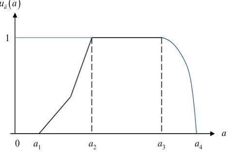
[12]. It is appropriate to recall here that a real fuzzy number a is a convex continuous fuzzy subset of the real line whose membership function µa

( )

a a, ∈R and satisfies the following properties:

1. A continuous mapping from R to the closed interval [0, 1]. 2.

µ

a

( )

a =0 for all a∈ −∞

(

,a1

]

.

(3)

4. µa

( )

a =1 for all a∈

[

a a2, 3

]

.

5. Strict decrease on

[

a a₃, ₄

]

. 6.

µ

a

( )

a =0 for all a∈

[

a4,+∞

)

.

A possible shape of fuzzy number p is illustrated inFigure 1.

Definition 1. (Dubois and Prade [12]).

The α-level set of the fuzzy numbers ai is defined as the ordinary set Lα

( )

a for which degree of their

membership function exceeds, the level α:

( )

{

| a

( )

i , 1, ,

}

Lα a = a

µ

 a ≥

α

i=  m

For a certain degree of α, the problem FMONLP can be rewritten by using Sakawa and Yano’s method [5]. In the following nonfuzzy α-multi-objective nonlinear programming problem form:

(α-MONLP) max

(

f x a1

(

, 1

) (

,f2 x a, 2

)

,,fm

(

x a, m

)

subject to x∈X a, ∈Lα

( )

a .

Problem (α-MONLP) can be rewritten as the following form:

(α-MONLP) max

(

f x a₁

(

, ₁

) (

,f₂ x a, ₂

)

,,fm

(

x a, m

)

subject to x∈X A, i≤ ≤ai B ii, =1,, ,m

where A Bi, i are lower and upper bounds on ai for i=1, 2,,m.

Indeed, Sakawa, and Yano [5] consider that the membership function µ_a_

( )

a is differentiable on

[

a a₁, ₄

]

and the problem FMONLP is stable, hence our new problem α-MONLP is also stable.

Definition 2. (α-Pareto optimal solution).

x∗∈X is said to be an α-Pareto optimal solution to the (α-MONLP), if and only if there does not exists another x∈X , a∈Lα

( )

a . Such that f x ai

(

, i

)

f x ai

(

, i

)

,i 1, 2, , ,m

∗ ∗

≥ =  with strictly inequality holding for at least one i, where the corresponding values of parameters a_i∗ are called α-level optimal parameters.

For some (unknown) implicit utility function we have the following problem: (αM) maxU

(

f₁

(

x a, ₁

) (

,f₂ x a, ₂

)

,,fm

(

x a, m

)



subject to x∈X, Ai≤ ≤ai Bi, i=1,, .m

where U (.) is a concave and continuously differentiable function. It is clear that

(

x a∗, ∗

)

is an α-Pareto optim-al solution of (α-MONLP) if and only if

(

x a∗, ∗

)

is optimal solution of (αM).

3. Stability Set of the First Kind [11]

In this section we discuss the stability set of the first kind of the nonlinear programming problem with fuzzy pa-rameters in the objective function.

[image:3.595.197.432.550.710.2]

Definition 3. (Stability set of the first kind).

Figure 1. Membership function of fuzzy number a.

( )

a a

µ

_

0 a₁ a₂ a₃ a₄

1

(4)

Suppose that

( )

, 2m

A B ∈R with a corresponding α-Pareto optimal solution

(

x a,

)

, then the stability set of the first kind of (α -MONLP) corresponding to

(

x a,

)

, denote by S x a

(

,

)

, is defined by

(

) (

{

)

2

(

)

(

)

}

, , m| , is an -Pareto optimal solution of -MONLP .

S x a = A B ∈R x a

α

Let a certain

( )

A B, with a corresponding α-Pareto optimal solution

(

x a,

)

be given, then from the stability of problem (α-MONLP) there exist.

(

)

2

, m

A B ∈R ,

ν

∈Rk, λ δ, and µ ∈Rm such that the following Kuhn-Tucker conditions are satisfied:

(

)

( )

1 1

, 0, 1, , ,

m k

j i

i j

i r j r

g f

x a x r n

x x λ ν = = ∂ ∂ + = = ∂ ∂

∑

 (1)

(

,

)

0, 1, , ,

i

i i i

i

f

x a i m

a

λ ∂ − +δ µ = =

∂  (2)

1 1, m i i λ = =

∑

(3)

( )

0, 1, , ,

j

g x ≤ j=  k (4)

0, 1, 2, , ,

i i

a −B ≤ i=  m (5)

0, 1, 2, , ,

i i

A − ≤a i=  m (6)

( )

0, 1, 2, ,

jgj x j k

ν = =  (7)

(

)

0, 1, , ,

i ai Bi i m

δ − = =  (8)

(

)

0, 1, 2, , ,

i Ai ai i m

µ − = =  (9)

, , , 0, 1, 2, , ; 1, 2, ,

i i i j i m j k

λ µ δ ν

≥ =  =  (10) The determination of the stability set of the first kind S x a

(

,

)

depends only whether any of the variables

, 1, , ,

i i m

δ

=  and any of the variables

µ

i,i=1, 2,, ,m given as Equation (2) and Equation (10), are

posi-tives or zero.

Given µi=0,i∈ ⊆I₁

{

1, 2,,m

}

;µi>0,i∉I₁, as Equation (2) and Equation (10), then in order that the

other Kuhn-Tucker conditions (6) and (9) yield

1 1

, ; , .

i i i i

A ≤a i∈I A =a i∉I

Given δi=0,i∈ ⊆I₂

{

1, 2,,m

}

;λi>0,i∉I₂, as Equation (2) and Equation (10), then in order that the

oth-er Kuhn-Tuckoth-er conditions (5) and (8) yield

2 2

, ; , .

i i i i

B ≥a i∈I B =a i∉I

Let

(

) (

{

)

}

1 2

2

, 1 1

2 2

, , | , ; ,

, ; ,

m

I I i i i i

i i i i

S x a A B R A a i I A a i I

B a i I B a i I

= ∈ ≤ ∈ = ∉

≥ ∈ = ∉

(

)

₁ ₂

(

)

1 2 , ,

, _{I I} ,

I I

S x a =



S x a

4. Problem Formulation

(5)

fol-lowing problem:

(

)

(

)

1 ₁

max min , ,

m l

ij i i i

i m

x X∈ ≤ ≤

∑

_i₌ w f x a − f

subject to x∈X a, ∈L_α

( )

a , i=1,, ,m

or equivalently

( )

l

W

α

maxη

subject to

(

)

1

, 0,1, 2, , ,

m

l h

ij i i

i

w z z h l

η

=

≤

∑

 − = 

( )

x a, ∈ ×X L_α

( )

a ,

where

(

)

1 ₁

min , ,

m l

ij i i i

i m_i w f x a f

η

≤ ≤ ₌

≈

∑

 − and w_ijl normalized trade-off weights for i≤ j

( )

1 , , j i l ij k j j i

U z U z

z z

w i j

U z U z

z z = ∂  ∂       _∂  _ _∂ _   = ≤ ∂  ∂       _∂  _ _∂ _  

∑



where z=

(

z z₁, ₂,,zm

)

,zi ≡ f x ai

(

, i

)

for i=1, 2,,m, and

(

, 1

)

, ,

(

,

)

l l l l l

l m m

z ≡ f x a  f x a . The following lemma establishes an important characteristic of the problem

α

Pl.

Lemma1.

Let

(

x a, ,η

)

be a solution for the problem

α

Wl, and let z =

(

fl

(

x a, ₁

)

,,fm

(

x a, m

)

. Then

(

x a,

)

is

an α-Pareto optimal solution to the α-MONLP problem.

Proof:

Suppose that

(

x a,

)

is not α-Pareto optimal solution, then there exists

(

x a∗, ∗

)

∈ ×X Lα

( )

a such that z∗ >z

and z∗≠z, where z

(

f₁

(

x a, ₁

)

, ,fm

(

x a, m

)

∗_≡ ∗ ∗ _ ∗ ∗ _{, then}

(

)

(

)

0,1, , ₁ 0,1, , ₁

min min

m m

l h l h

ij ij

h l_i w z z h l_i w z z

η ∗

= ₌ = ₌

=

∑

− <

∑

−

    ,

which contradicts with the optimality of

(

x a, ,η

)

. This completes the proof.

5. Interactive Algorithm

Following the above discussion, the interactive algorithm to derive the satisficing solution for the DM from among the α-Pareto optimal solution set is constructed. The steps are marked with numbers involving interaction with the DM.

Step 1: Ask the DM to select the initial values of α, 0

(

≤ ≤α 1

)

. Step 2: Determine the α-level set of the fuzzy numbers.

Step 3: Convert the FMONLP in the form of α-MONLP and select an initial feasible point

(

x al, l

)

, set l = 0 and let zl=

(

fl

(

x al, ₁l

)

,,fm

(

x al, ml

)

.

Step 4: The DM specify values of wijl at

(

,

)

l l

x a for i=1, 2,,m.

Step 5: Solve problem

α

Wl. Suppose

(

xl+1,al+1,

η

l+1

)

be an optimal solution, and let

(

)

(

)

(

)

1 1 1 1 1

1

, , , ,

l l l l l

l m m

z+ = f x+ a+  f x+ a+ . Set l = l + 1. Step 6: If η =l 0, go to Step 7. Otherwise go to Step 4. Step 7: Determine the stability set of the first kind S x a

(

,

)

.

Step 8: If the DM is satisfied with the current values of the objective functions and α of α-Pareto solution, go to Step 9. Otherwise, ask the DM to update the degree α and return to Step 2.

Step 9: Terminate with

(

l, l

)

(6)

6. Numerical Illustration Example

In this section, we give an example to illustrate the theoretical part have mention above. Our computation is car-ried out by utilizing MAPLE 13 (see Appendix).

Consider the following fuzzy multi-objective nonlinear programming problem (FMONLP) max

(

x₁+a x₁, ₂+a₂

)

subject to x∈ =X

{

(

x x₁, ₂

)

|− +x₁ x₂≤3,x₁2+x₂2 ≤25, ,x x₁ ₂≥0

}

, with

( )

1

1 2

2 1

2 3

4

3 4

4

0

1

0

i

a i i

i

a c

c a c

c c

a c a c

a c

c a c

c c

c a

µ

− ∞ < ≤ 

 −

 _< _<

 − 

=_ ≤ ≤

 −

 < <

− 

 _≤ _{< ∞}

 

where I = 1, 2 and the values of cj,

(

j=1, 2, 3, 4

)

are given as in the following table:

i

a c1 c2 c3 c4

1

a 3.8 4 4.8 5

2

a 1 2 3 4

Let z₁= f₁

(

x a, ₁

)

= +x₁ a₁ and z₂= f₂

(

x a, ₂

)

=x₂+a₂. The DM’s utility function U is assumed to be as the following:

(

)

2

(

)

2

1 20 2 2 10

U = − z − − z −

Step 1: Suppose that the DM select α = 0.9.

Step 2: L0.9

( ) (

a =

{

a a1, 2

)

| 3.98≤a1≤4.82 and 1.9≤a2 ≤3.1

}

Step 3: The α-MONLP problem becomes:

(

1 1 2 2

)

max x +a x, +a

subject to x∈X a, ∈L_0.9

( )

a

Let us select the feasible point

(

x a0, 0

)

=

(

3.18, 2.9, 4.82, 3.1

)

as the starting solution. Hence, the corres-ponding point in the objective space is: z0≡

( )

8, 6 .

Step 4: The normalized trade off weights w0 at

(

x a0, 0

)

is: w0 =

(

0.6, 0.4

)

. Step 5: Solve the following problem:

(

0

)

W

α

maxη

subject to

η

≤0.6x₁+0.4x₂+0.6a₁+0.4a₂−7.2

( )

0.9

,

x∈X a∈L a

The outputs of our calculation are show in Table 1. Step 6: Since η ≠l 0, then return to Step 4.

Repeat Steps 4 - 6 till η ≈l 0, otherwise, go to Step 7. Step 7: The corresponding stability set of the first kind is:

(

9 9

)

{

(

)

}

1 1 2 2

, , | 4.82, 4.82, 3.1, 3.1 .

S x a = A B A ≤ B = A ≤ B =

(7)

[image:7.595.82.539.88.253.2]

Table 1. The solution of the problem

(

l

)

, 1, 2, ,9

W l

α =  .

Iteration l

(

_{x a}l, l

)

ηl l

z

1 (4.16025, 2.7735, 4.82, 3.1 ) 0.53755 (8.98025, 5.8735 ) 2 (4.003358, 2.9955173, 4.82, 3.1 ) 0.00528124 (8.823358, 6.0955173 ) 3 (4.1004068, 2.8612347, 4.82, 3.1 ) 0.0019716 (8.9204068, 5.9612347 ) 4 (4.038235, 2.948331, 4.82, 3.1 ) 0.0008195 (8.858235, 6.048331 ) 5 (4.078066, 2.892987, 4.82, 3.1 ) 0.00033366 (8.898066, 5.992987 ) 6 (4.0497106, 2.93254906, 4.82, 3.1 ) 0.0001699 (8.8697106, 6.03254906 ) 7 (4.0724333, 2.9009114, 4.82, 3.1 ) 0.000108795 (8.8924333, 6.0009114 ) 8 (4.0554198, 2.9246487, 4.82, 3.1 ) 0.0000611 (8.8754198, 6.0246487 ) 9 (4.0665451, 2.9091599, 4.82, 3.1 ) ≈0 (8.8865451, 6.0091599 )

Step 9: The final solution is

(

x a9, 9

)

=

(

4.0665451, 2.9091599, 4.82, 3.1

)

.

7. Conclusions

In this paper we have integrated different methods like normalized trade-off in [9] and compromised method by Kassem [11] to find a modified method which can be used to solve and obtain an optimal solution to the as-sumed problem.

The modified technique is based on the reformulation of the given problem and in such way that enables us to solve it easily. A new form of the assumed problem is obtained; hence using a computer program the stability of its solution is studied. Moreover, depending on stability calculation, the validity of the optimal solution has been ensured.

References

[1] Shih, C.J. and Lee, H.W. (2004) Level-Cut Approaches of First and Second Kind for Unique Solution Design in Fuzzy Engineering Optimization Problems. Tamkang Journal of Science and Engineering, 7, 189-198.

[2] Osman, M. (1977) Qualitative Analysis of Basic Notions in Parametric Convex Programming I (Parameters in the Constraints). Aplikace Matematiky, 22, 318-332.

[3] Osman, M. and El-Banna, A. (1993) Stability of Multiobjective Nonlinear Programming Problems with Fuzzy Para-meters. Mathematics and Computers in Simulation, 35, 321-326. http://dx.doi.org/10.1016/0378-4754(93)90062-Y

[4] Kassem, M. (1995) Interactive Stability of Multiobjective Nonlinear Programming Problems with Fuzzy Parameters in the Constraints. Fuzzy Sets and Systems, 73, 235-243. http://dx.doi.org/10.1016/0165-0114(94)00317-Z

[5] Sakawa, M. and Yano, H. (1989) Interactive Decision Making for Multiobjective Nonlinear Programming Problems with Fuzzy Parameters. Fuzzy Sets and Systems, 29, 315-326. http://dx.doi.org/10.1016/0165-0114(89)90043-2

[6] Katagiri, H. and Sakawa, M. (2011) Interactive Multiobjective Fuzzy Random Programming through the Level Set- Based Probability Model. Information Sciences, 181, 1641-1650. http://dx.doi.org/10.1016/j.ins.2011.01.003

[7] Loganathan, G.V. and Sherali, H.D. (1987) A Convergent Interactive Cutting-Plane Algorithmfor Multiobjective Op-timization. Operations Research, 35, 365-377.

[8] Jameel, A. and Sadeghi, A. (2012) Solving Nonlinear Programming Problem in Fuzzy Enlivenment. International Journal of Contemporary Mathematical Sciences, 7, 159-170.

[9] Elshafei, M.M. (2006) Interactive Stability of Multiobjective Integer Nonlinear Programming Problems. Applied Ma-thematics and Computation, 176, 230-236.

[10] Pendharkar, P.C. (2013) Scatter Search Based Interactive Multi-Criteria Optimization of Fuzzy Objectives for Coal Production Planning. Engineering Applications of Artificial Intelligence, 26, 1503-1511.

http://dx.doi.org/10.1016/j.engappai.2013.01.001

[11] Kassem, M. (2007) Interactive Stability Cutting-Plane Algorithm for Multiobjective Nonlinear Programming Problems. Applied Mathematics and Computation, 192, 446-456. http://dx.doi.org/10.1016/j.amc.2007.03.037

(8)

Appendix

A maple program for solving multi-objective nonlinear programming (MONLP) problems and stability of this solution. >restart:

With (Optimization):

>N1: = solve ({(a[1] − 3.8)/(4 − 3.8)> = 0.9}, [a[1]]); >N2: = solve ({(a[1] − 5)/(4.8 − 5)> = 0.9}, [a[1]]); N3: = solve ({(a[2] − 1)/(2 − 1)> = 0.9}, [a[2]]);

>N4: = solve ({(a[2] − 4)/(3 − 4)> = 0.9}, [a[2]]);

>U: = - (z[1] − 20) ^ 2 – 2 * (z[2] − 10) ^ 2; r[1]: = diff (U, z[1])/(diff (U, z[1]) + diff (U, z[2])); r[2]: = diff (U, z[2])/(diff (U, z[1]) + diff (U, z[2])); r[1]: = sub s ({z[1] = 3.18 + 4.82, z[2] = 2.9 + 3.1}, r[1]); r[2]: = subs ({z[1] = 3.18 + 4.82, z[2] = 2.9 + 3.1}, r[2]);

Q1: = Maximize (e, {e < = 0.6 * a[1] + 0.6 * x[1] + 0.4 * a[2] + 0.4* x[2] − 7.2, −x[1] + x[2] < = 3, x[1] ^ 2 + x[2] ^ 2 < = 25, 3.98 < = a[1], a[1] < = 4.82, 1.9 < = a[2], a[2] < = 3.1}, assume = nonnegative);

r[1]: = diff (U, z[1])/(diff (U, z[1]) + diff (U, z[2])); r[2]: = diff (U, z[2])/(diff (U, z[1]) + diff (U, z[2]));

r[1]: = subs ({z[1] = 4.16025 + 4.82, z[2] = 2.7735 + 3.1}, r[1]); r[2]: = subs ({z[1] = 4.16025 + 4.82, z[2] = 2.7735 + 3.1}, r[2]);

Q2: = Maximize(e, {e < = 0.572 * x[1] + 0.428 * x[2] + 0.572 * a[1] + 0.428 * a[2] − ((0.572 * 8.98025) + (0.428 * 5.8735)), −x[1] + x[2] < = 3, x[1] ^ 2 + x[2] ^ 2 < = 25, 3.98 < = a[1], a[1] < = 4.82, 1.9 < = a[2], a[2] < = 3.1}, assume = nonnegative);

r[1]: = diff (U, z[1])/(diff(U, z[1]) + diff (U, z[2])); r[2]: = diff (U, z[2])/(diff(U, z[1]) + diff (U, z[2]));

Q3: = Maximize (e, {e < = 0.589 * x[1] + 0.411 * x[2] + 0.589 * a[1] + 0.411 * a[2] − ((0.589 * 8.823358) + (0.411 * 6.0955173)), −x[1] + x[2] < = 3, x[1] ^ 2 + x[2] ^ 2 < = 25, 3.98 < = a[1], a[1] < = 4.82, 1.9 < = a[2], a[2] < = 3.1}, assume = nonnegative);

r[1]: = diff (U, z[1])/(diff (U, z[1]) + diff (U, z[2])); r[2]: = diff (U, z[2])/(diff (U, z[1]) + diff (U, z[2]));

Q4: = Maximize (e, {e < = 0.578 * x[1] + 0.422 * x[2] + 0.578 * a[1] + 0.422* a[2] − ((0.578 * 8.9204068) + (0.422 * 5.9612347)), −x[1] + x[2] < = 3, x[1] ^ 2 + x[2] ^ 2 < = 25, 3.98 < = a[1], a[1] < = 4.82, 1.9 <= a[2], a[2] < = 3.1}, assume = nonnegative);

r[1]: = diff (U, z[1])/(diff(U, z[1]) + diff (U, z[2])); r[2]: = diff (U, z[2])/(diff(U, z[1]) + diff (U, z[2]));

Q5: = Maximize (e, {e< = 0.585 * x[1] + 0.415 * x[2] + 0.585 * a[1] + 0.415 * a[2] − ((0.585 * 8.858235) + (0.415 *

6.048331)), −x[1] + x[2] < = 3, x[1] ^ 2 + x[2] ^ 2 < = 25, 3.98 < = a[1], a[1] < = 4.82, 1.9 < = a[2], a[2] < = 3.1}, assume = nonnegative);

>r[1]: = diff (U, z[1])/(diff (U, z[1]) + diff (U, z[2])); r[2]: = diff (U, z[2])/(diff (U, z[1]) + diff (U, z[2]));

r[1]: = subs ({z[1] = 4.078066 + 4.82, z[2] = 2.892987 + 3.1}, r[1]); r[2]: = subs ({z[1] = 4.078066 + 4.82, z[2] = 2.892987 + 3.1}, r[2]);

Q6: = Maximize (e, {e < = 0.58 * x[1] + 0.42 * x[2] + 0.58 * a[1] + 0.42 * a[2] − ((0.58 * 8.898066) + (0.42 * 5.992987)),

−x[1] + x[2] < = 3, x[1] ^ 2 + x[2] ^ 2 < = 25, 3.98 < = a[1], a[1] < = 4.82, 1.9 < = a[2], a[2] < = 3.1}, assume = nonnega-tive);

(9)

r[1]: = subs ({z[1] = 4.0497106 + 4.82, z[2] = 2.93254906 + 3.1}, r[1]); r[2]: = subs ({z[1] = 4.0497106 + 4.82, z[2] = 2.93254906 + 3.1}, r[2]);

Q7: = Maximize (e, {e < = 0.584 * x[1] + 0.416 * x[2] + 0.584 * a[1] + 0.416 * a[2] − ((0.584 * 8.8697106) + (0.416 *

6.03254906)), −x[1] + x[2] < = 3, x[1] ^ 2 + x[2] ^ 2 < = 25, 3.98 < = a[1], a[1] < = 4.82, 1.9 < = a[2], a[2] < = 3.1}, as-sume = nonnegative);

>r[1]: = diff (U, z[1])/(diff (U, z[1]) + diff (U, z[2])); r[2]: = diff (U, z[2])/(diff (U, z[1]) + diff (U, z[2]));

Q8: = Maximize (e, {e < = 0.581 * x[1] + 0.419 * x[2] + 0.581 * a[1] + 0.419 * a[2] − ((0.581 * 8.8924333) + (0.419 * 6.0009114)), −x[1] + x[2] < = 3, x[1] ^ 2 + x[2] ^ 2 < = 25, 3.98 < = a[1], a[1] < = 4.82, 1.9 < = a[2], a[2] < = 3.1}, assume = nonnegative);

>r[1]: = diff(U, z[1])/(diff (U, z[1]) + diff (U, z[2])); r[2]: = diff (U, z[2])/(diff (U, z[1]) + diff (U, z[2]));

Q9: = Maximize (e, {e < = 0.583 * x[1] + 0.417 * x[2] + 0.583 * a[1] + 0.417 * a[2] − ((0.583 * 8.8754198) + (0.417 *