Munich Personal RePEc Archive
Garch Parameter Estimation Using
High-Frequency Data
Visser, Marcel P.
Korteweg-de Vries Instute for Mathematics, University of
Amsterdam
10 June 2008
Online at
https://mpra.ub.uni-muenchen.de/9076/
Garch Parameter Estimation
Using High-Frequency Data
Marcel P. Visser
∗June 10, 2008
Abstract
Estimation of the parameters of Garch models for financial data is typically based on daily close-to-close returns. This paper shows that the efficiency of the parameter estimators may be greatly improved by using volatility proxies based on intraday data. The paper develops a Garch quasi maximum likelihood estimator (QMLE) based on these proxies. Examples of such proxies are the realized volatility and the intraday high-low range. Empirical analysis of the S&P 500 index tick data shows that the use of a suitable proxy may reduce the variances of the estimators of the Garch autoregression parameters by a factor 20.
JEL classification: C14, C22, C51, G1.
Key Words: volatility estimation, quasi maximum likelihood, volatility proxy, Gaussian
QMLE, log-Gaussian QMLE, autoregressive conditional heteroscedasticity.
∗Korteweg-de Vries Institute for Mathematics, University of Amsterdam. Plantage Muidergracht 24,
1
Introduction
Garch models based on close-to-close daily returns do quite well in describing financial volatil-ity, but they seem incompatible with intraday high-frequency data at first sight. The standard continuous time model for the log of asset prices is a semimartingale, and volatility is then the square root of the quadratic variation process. High-frequency data are accordingly used to estimate the daily increment in the quadratic variation. In the discrete time setting of Garch models, the day volatility is the scale factor that transforms the iid innovationZn into
the log-return rn.
Throughout this paper we assume that the sequence of daily log-returns rn is a
sta-tionary Garch(1,1) process. We use the Garch(1,1) representation given by Drost and Klaassen (1997):
rn = vnτ Zn (1)
vn2 = 1 +γr2n−1 +βv2n−1, (2)
where the innovations Zn are iid, mean zero. For identification the second moment is
stan-dardized by EZ2
n = 1. This system is equivalent to the more familiar Garch equations
rn = σnZn and σn2 = κ+αrn2−1 +βσn2−1 by writing σn = vnτ, and κ = τ2, α = γτ2. The
system given by (1) and (2) has the advantage that the standardization of Zn affects only
the norming parameter τ.The focus on Garch(1,1) is for simplicity of exposition only. The principle below allows one to improve estimation of the parameters of any scale process vn.
Let us say a few words on parameter estimation in this model. The returns rn, n =
1, . . . , N, are observable, the volatilities vn are not. One may estimate the parameter θ =
(τ, γ, β) in (1) and (2) by maximizing the log-likelihood of the observations rn. If the Zn are
standard Gaussian, one obtains the likelihood by using that the returns rn are conditionally
Gaussian distributed with mean zero and variance v2
nτ2. If the distribution of the random
variables Zn is unknown, one may still proceed as if the Zn were standard Gaussian. The
estimator is then called a quasi-ML estimator (QMLE).
(1997). One may also start from a continuous time diffusion. The discretized process is then a stochastic volatility model and one may use the high-low range for parameter estimation, see Alizadeh, Brandt and Diebold (2002). If the diffusion coefficient is an Ornstein-Uhlenbeck process, or a CEV process, then the daily integrated volatility is an ARMA(1,1) process. The ARMA parameters may then be estimated by state space methods, see Barndorff-Nielsen and Shephard (2002).
The present paper takes a different approach. We start out from the Garch system (1) and (2) for the daily close-to-close returns rn. For each day n we observe the entire intraday
log-return process Rn(·). To distill the day volatility fromRnone may use the empirical realized
quadratic variation RQVn based on five-minute intervals (also called realized variance). One
obtains RQVn by summing the squared five-minute increments over the n-th trading day.
The realized volatility Hn = √RQVn is generally seen as a good proxy for volatility. Now,
the parameters γ and β play a role in the likelihood for the Hn. If one could construct
this likelihood, one hopes to find an efficiency gain compared with estimation based on the likelihood for the returnsrn. To obtain the likelihood for the proxiesHnone needs to embed
the close-to-close return rn in a model for the intraday return process Rn. As a model we
shall propose a simple extension of the daily Garch process to a continuous time intraday log-return process Rn. This intraday extension yields the following system for the volatility
proxy Hn:
Hn = vnτH ZH,n (3)
vn2 = 1 +γr2n−1+βv2n−1, (4)
where the innovations ZH,n ≥ 0 are iid and have standardization EZH,n2 = 1. The system
given by (3) and (4) has the property that the parameters γ, β in (4) have the same value as in equation (2). So Hn and rn share the daily factor vn. We derive the likelihood for
the observations Hn and show how one may estimate the parameter θ = (τH, γ, β) by quasi
maximum likelihood. More generally, we shall show that one may replaceHnby other proxies
than the realized volatility; for example the intraday high-low range, or the absolute value of the maximal decrease ofRn over a fifteen minute interval.
The theory developed in the paper gives exact relationships for the asymptotic relative efficiency of QML estimators for γ and β using alternative proxies Hn. The quality of the
estimator is determined by the innovation ZH.If the variance of ZH2 is smaller than var(Z2),
then the QML estimator for γ, β based on the proxies Hn is sharper than the one based
based onHn. Its proof is based on the likelihood theory in Straumann and Mikosch (2006).
A similar estimation theory may be developed using the log proxies, log(Hn).
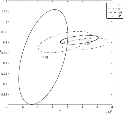
The estimators are applied to the four years 1992–1995 of the S&P 500 index. We motivate this choice of time period in Section 4. We emphasize that it is not our aim to identify an optimal volatility model. For using volatility proxies as predictors of future volatility we refer to Engle and Gallo (2006) and Ghysels, Santa-Clara, and Valkanov (2006). The purpose of the present analysis is to judge the potential benefits of using volatility proxies based on intraday data for parameter estimation. Figure 1 gives an impression of the empirical efficiency gains. It shows four 95% confidence ellipses for estimates of (γ, β), based on |rn|
−1 0 1 2 3 4 5 6
x 104 0.65
0.7 0.75 0.8 0.85 0.9 0.95 1 1.05 1.1
|r|
hl
rv5 H*
γ β
[image:5.595.188.396.259.452.2]|r| hl rv5 H*
Figure 1: Confidence regions for estimators of (γ, β), based on alternative volatility proxiesH. The data are the S&P 500 index futures over 1992–01–01 to 1995–12–31 (1001 days). In the figure |r| depicts the Gaussian QMLE applied to the absolute returns|rn|(the usual Garch(1,1) QMLE). The other estimates are based on the log-Gaussian QMLE applied tohl (high-low range), RV5 (five-minute realized volatility) and
H∗ (a proxy determined in de Vilder and Visser (2007)).
and on three other proxies. The confidence regions are computed using Bollerslev-Wooldridge (1992) robust covariances. The main point of this paper is made in the figure: one may greatly improve the parameter estimation for Garch processes by the use of suitable proxies based on high-frequency data.
Section 4 applies the QMLE’s to the S&P 500 index data. Section 5 compares simulations for estimators of (γ, β) based on realized variance with the standard QMLE based on close-to-close returns. Our conclusions are presented in Section 6. Appendices A, B, C, and D give a description of the data, background on QML estimation, proofs, and background on simulations.
2
Preliminaries
Section 2.1 introduces the model for the intraday return process Rn(·). Section 2.2
char-acterizes the volatility proxies that may be used for QML estimation. For a more detailed account of the model forRn, and of proxies, see de Vilder and Visser (2007).
2.1
Intraday Return Process
To deal with high-frequency data in the daily Garch system given by (1) and (2) one needs to embed the sequence of daily close-to-close returns (rn) in a continuous time process. Each day
we observe the continuous time, intraday log-return process Rn(·): observable information
is the filtration (Fn), given by σ(Rk, k ≤ n). The process Rn represents within day n the
log-return with respect to the previous day’s close. DescribeRn(·) as the product of the scale
factor vnτ and a cadlag1 process Ψn(·) on the time interval [0,1], the trading day:
Rn(u) =vnτ Ψn(u), 0≤u≤1,
where the processes Ψn(·) are iid over different days, have standardization EΨ2n(1) = 1, and
intraday time u advances from zero to one. So Rn(0) gives the overnight return and Rn(1)
equals the close-to-close return rn. The scale factor vnτ is the same as in the discrete time
model (1), and is constant within the day. The process Ψn may be any process representing
the intraday price pattern. This continuous time model is simple enough to allow for analysis, and it takes into account the diversity in the behaviour of the market on successive trading days. One may recover the close-to-close returnsrn by setting Zn= Ψn(1) :
rn=Rn(1) =vnτ Zn.
2.2
Volatility Proxies
Let us introduce proxies for the volatility vnτ. In general we call the random variable Hn =
H(Rn) (or the functional H) aproxy whenever H is positive and is positively homogeneous
inRn. Positive homogeneity means:
H(sRn) =sH(Rn), s≥0. (5)
The absolute return|rn| is a proxy. Other examples are the intraday high-low range and the
realized volatility.
We assume that the random variable H(Ψ) is not identically zero,
µH2 =
p
EH2(Ψ)>0.
Let us introduce the normalized innovation ZH by setting
ZH =H(Ψ)/µH2,
so EZ2
H = 1. By homogeneity Hn =H(Rn) =vnτ H(Ψn),which gives (cf. (3))
Hn =vnτHZH,n,
where the positive, iid innovationsZH,n ≥0 have EZH2 = 1, and τH =τ µH2 .Replacing H by
3H only adds a factor 3 to the norming parameter τH. A good proxy H distills the factor
vnτH fromRn without much error.
3
QML Estimators Based on a General Volatility
Mea-sure
This section develops the theory for estimation of the parametersγandβusing the proxyHn,
as sketched in the introduction. We first treat the Gaussian QML estimator, which is based on the multiplicative equation Hn =vnτHZH,n.We then discuss the log-Gaussian QMLE, which
is a Gaussian QMLE applied to the additive equation log(Hn) = log(vn)+log(τH)+log(ZH,n).
Let us address one important issue first. Why should one bother with likelihood methods if one can simply obtain v2
nτ2 from the intraday return process Rn(·)? Consider for example
intraday returns, as the length of the sampling intervals approach zero. If the process Ψ(·) of Section 2.1 is a Brownian motion, then QV(Ψ) = 1, so QV(Rn) =vn2τ2.In general we do
not have this exact relationship. Under fairly mild conditions the quadratic variation of Rn
is an unbiased estimator of the conditional variance of the daily return,
E(QVn|Fn−1) = var(rn|Fn−1) =vn2τ2,
see for instance Andersen, Bollerslev, Diebold, and Labys (2003). GenerallyQVn 6= var(rn|Fn−1)
so the conditional variancev2
nτ2 remains unobservable. If one happens to be in the fortunate
circumstance of having a perfect proxy, Hn =vnτH, then the QML estimation below yields
perfect estimates. A second reason for considering likelihood methods is that one may want to study the dynamics of a sequence of proxies (Hn). These dynamics are determined by the
volatilities (vn). So the (vn) are central to understanding the time series behaviour of, for
example, the realized volatilities RVn.
3.1
Gaussian QMLE
This section extends the usual Garch QMLE based on close-to-close returns to a QMLE based on the proxies Hn. For a brief review of the Garch(1,1) QMLE based on close-to-close
returns, see Appendix B.3.
Recall that the intraday return process Rn(·) = vnτΨn(·) yields close-to-close returns
rn=vnτ Zn. From Section 2.2 we know that the volatility proxy Hn satisfies
Hn =vnτHZH,n. (6)
Similarly to the case of squared returns one has the relationE(H2
n|Fn−1) =vn2τH2.The
volatil-ity dynamics (vn) and the autoregression parameters (γ, β) are the same as those forrn.The
norming parameter τ0
H is related toτ0 for the returns rn by
τH0 =τ0µH2 , (7)
reflecting that the overall scale ofHnmay differ from the overall scale of the absolute returns |rn|. The principle of quasi maximum likelihood may be applied to the multiplicative
equa-tion (6). First consider the absolute returns |rn|. Treating these as absolute values of mean
zero Gaussian random variables gives the same likelihood as simply treating the returnsrn as
set the observation yn = |rn|, the conditional mean µn = 0, and the conditional variance
hn = v2nτ2, since the Gaussian log-likelihood needs the value for yn2 = rn2 only, and not the
value ofrn:
LN(θ; y1, . . . , yN) =−
1 2
N
X
n=1
log(v2n(γ, β)τ2) +
y2
n
v2
n(γ, β)τ2
, (8)
modulo an unimportant constant.
Similarly, treating Hn as if it were the absolute value of a mean zero Gaussian
ran-dom variable yields a QML estimator for (τH, γ, β). So one may set yn = Hn, µn = 0, and
hn =v2nτH2,to obtain the QMLE ˆθN.We refer to this QMLE as theGaussian QMLE (based
onHn).
For notational convenience we write
σH,n =vnτH. (9)
Equation (9) suppresses the parameter θ in σH,n = σH,n(θ) for θ = (τH, γ, β). Define the
matrix GH by
GH(θ)i,j =E
1
σ4
H,0(θ)
∂ σ2
H,0(θ)
∂θi
∂ σ2
H,0(θ)
∂θj
. (10)
The QML covariance matrix V0, Appendix B.1 equation (28), now simplifies to the matrix
given in (12). One obtains the regularity conditions for the Gaussian QMLE by adjusting the six conditions of Appendix B.3 for the QMLE based on close-to-close returns. One has to adjust the condition EZ4 <∞ to EZH4 < ∞, and replace τ by τH in condition (2). One
has to keep τ0 in condition (3). This yields the following assumptions:
A1. (Zn) is an iid sequence with EZ2 = 1,
A2. τH >0, γ > 0, β ∈[0,1),
A3. Elog (γ0(τ0)2Z2+β0)<0 ,
A4. Z2 is non-degenerate,
A5. EZ4
A6. P(|Z| ≤z) =o(zµ) as z ↓0,for some µ >0.
The only condition that concerns ZH is (A5). Most conditions concern the innovation Z of
the close-to-close returns rn. This is because Zn appears in the volatility process vn, which
is driven by the close-to-close returns. For more background on the conditions (A1) to (A6), see Appendix B.3.
Theorem 3.1. Let θ0 = (τ0
H, γ0, β0) and τH0 = τ0µH2 , see equation (7). Assume conditions
(A1) to (A6). Then the Gaussian QMLE θˆN is asymptotically normal:
√
N(ˆθN −θ0) d
→ N(0, V0), N → ∞, (11)
with
V0 = var(ZH2) G−H1(θ
0). (12)
The proof of Theorem 3.1 consists of an adjustment of the proof of Straumann and Mikosch (2006) for the QMLE based on the returns yn=rn to the case that yn=Hn. One may find
it in Appendix C.
Let us recall the notion of asymptotic relative efficiency. If two competing estimators ˆ
φ(1)N and ˆφ(2)N are consistent and asymptotically normal estimators of a parameter φ with asymptotic variances (σφ(1))2 and (σ(2)
φ )2, then the asymptotic relative efficiency (ARE) is
given by
ARE = (σφ(1))2/(σφ(2))2.
The following lemma enables the comparison of the QML covariance matricesV0 for
estima-tors of γ and β based on alternative proxies H.The proof may be found in Appendix C.
Lemma 3.2. The (γ, β)-block of G−1
H (θ0) in Theorem 3.1 does not depend on the particular
proxy H.
Corollary 3.3 below follows from Theorem 3.1 and Lemma 3.2.
Corollary 3.3. Consider two Gaussian QMLE’s for γ and β from Theorem 3.1, the first
based on proxies H′
efficiency
AREGaussian(H′, H) =
var(ZH2′)
var(Z2
H)
. (13)
As a final remark, suppose that the volatilitiesvn are a scale process other than Garch(1,1).
One may then still extend the daily returns rn to Rn(·) = vnτΨn(·), and obtain results
analogous to the results in the present section.
3.2
Log-Gaussian QMLE
One may also estimate the parameters (γ, β) of the Garch system given by (1) and (2) by a log-Gaussian QMLE. This section develops the log-Gaussian QMLE, similarly to the Gaus-sian QMLE. Readers may prefer to skip Sections 3.2 to 3.4 upon first reading, and proceed directly to the empirical results of Section 4.
The log-Gaussian QMLE consists of applying Gaussian quasi maximum likelihood to the log proxies log(Hn). Applying logarithms to Hn yields the equation log(Hn) = log(vn) +
log(τH) + log(ZH,n).Define ˜τH =τHexp(Elog(ZH,n)), and
UH,n=
log(ZH,n)−Elog(ZH,n)
p
var(log(ZH,n))
.
We may now write the additive equation
log(Hn) = log(vn) + log(˜τH) +λUH,n, (14)
where the errors UH,n are iid(0,1). The system (14) yields E(log(Hn)|Fn−1) = log(vn) +
log(˜τH),and var(log(Hn)|Fn−1) =λ2.The parameterλ2 represents the measurement variance
of log(Hn), a proxy for log volatility, with
(λ0)2 = var(log(ZH)).
Define ˜θ= (˜τH, γ, β) and define the extended parameter
η= (˜θ, λ).
QMLE of Section 3.1. The additive equation (14) fits into the framework of quasi maximum likelihood estimation (see Appendix B.1), setting yn = log(Hn), µn(η) = log(σH,n(˜θ)) and
hn(η) =λ2.We refer to the maximizer ˆηN as the log-Gaussian QMLE. Let us determine the
QML covariance matrixV0 of Appendix B.1. The matrixA0 is block diagonal since the mean
and variance functions do not share parameters. Applying
∂µn(η)
∂ηi
= 1
2σ2
H,n(˜θ)
∂σH,n2 (˜θ)
∂ηi
,
one finds that the ˜θ-block and the diagonal element for λ of A0 satisfy
(A0)θ˜=
1
4(λ0)2GH(˜θ
0), (A 0)λ =
2 (λ0)2,
with GH given by equation (10). The ˜θ-block of B0 equals the ˜θ-block of A0, the diagonal
element for λ equals (B0)λ = (λ10)2var(UH2). The off-diagonal (˜θ, λ)-column of B0 equals
(B0)θ,λ˜ = 1
(λ0)2EU 3
H E
∂µn
∂θ˜(˜θ
0)′,
making use of µn(η) = µn(˜θ). The covariance matrix V0 = A−01B0A−01 divided into (˜θ, λ
)-blocks now reads
V0 = 4(λ0)2
G−1
H (˜θ0) 12EUH3 E ∂µn
∂θ˜ (˜θ
0)′
1 2EU
3
H E
∂µn
∂θ˜(˜θ
0) 1 16var(U
2
H)
!
. (15)
Assume conditions (A1) to (A6) and replace condition (A5) by
A5’. E(log(ZH))4 <∞.
The QML theory of Appendix B.1 suggests that the log-Gaussian QMLE ˆηN is asymptotically
normal,
√
N(ˆηN −η0)
d
→ N(0, V0), N → ∞, (16)
with V0 the covariance matrix given by (15), though we do not produce a formal proof
like the proof of Theorem 3.1. The covariance matrix (15) makes clear that the smaller (λ0)2 = var(log(Z
H)) the more efficient the QMLE for γ and for β. Similarly to Corollary
different proxies H′
n and Hn is given by
ARElog-Gaussian(H′, H) =
var(log(ZH′))
var(log(ZH))
. (17)
De Vilder and Visser (2007) define an optimal proxy H∗ as a proxy with minimal variance
of the logarithm,
var(log(H∗(Ψ))) = inf
H var(log(H(Ψ))).
Such an optimal proxy also yields the most efficient log-Gaussian QMLE forγ and β.
We end this section with a remark that is relevant to practical implementation of the log-Gaussian QMLE. The numerical value of ˆλ does not influence the numerical values of the parameters in ˜θ. This is due to the usual effect that the value of the variance parameter does not influence the value of the mean parameter for Gaussian QML (this is true if the variance function and the mean function do not share parameters). Moreover, the usual ‘sandwich’ QML covariance matrix ˆV estimated by plugging in ˆA and ˆB in equation (28), also does not depend on the numerical value of ˆλ as far as the ˜θ-parameters are concerned. So the value of ˆλ is irrelevant to inference on ˜θ.
3.3
Efficiency of log-Gaussian QMLE versus Gaussian QMLE
Let us briefly compare the asymptotic efficiency of ˆγ,βˆ for the log-Gaussian and Gaussian QMLE. Comparing the (γ, β)-blocks of V0 in equations (12) and (15), one finds that the
asymptotic relative efficiency of the log-Gaussian and Gaussian QMLE’s for γ and β,based on the same proxy Hn is given by
ARE(log-Gaussian,Gaussian) = 4var(log(ZH)) var(Z2
H)
. (18)
So, the log-Gaussian QMLE is more efficient if 4(λ0)2 = var(log(Z2
H)) ≤ var(ZH2), where
EZ2
H = 1.This inequality does not always hold: var(log(ZH)) may be large if ZH has values
close to zero, while var(Z2
H) may be large if ZH has heavy tails. The following example
considers the case that ZH has a lognormal distribution.
Example 3.3.1. LetZH have a lognormal(−σ2, σ2)distribution. Thenlog(ZH)∼ N(−σ2, σ2).
Thej-th moment of a lognormal(µ, σ2)equalsejµ+j2
σ2
/2, soEZ2
H = 1 andvar(ZH2) =e4σ
2
Apply relation (18) to find
ARE(log-Gaussian,Gaussian) = 4σ
2
e4σ2
−1.
Since 4σ4 ≤ e4σ2
−1 the log-Gaussian QMLE is more efficient for all values of σ2. In this
example the log-Gaussian QMLE is the exact maximum likelihood estimator.
3.4
Relative Error of Volatility Extraction
One may also be interested in the quality of the estimator of the scale factorσH,n=vnτH,for
some fixed n. The volatility extraction θ→ σˆH,n(θ), with initialization ˆv0 is a function of θ.
To simplify the notation we omit the hat onσH,n in this section. If we plug in the estimator
ˆ
θN, we obtain the estimated volatility extraction σH,n(ˆθN). The asymptotic distribution of
σH,n(ˆθN) for N → ∞ may be found by the Delta method. Let the row vector ˙σH,n denote
the derivative of σH,n with respect to θ. Let V0 denote the asymptotic covariance matrix of
θ.The Delta method gives
√
N(σH,n(ˆθN)−σH,n(θ0))→ N( 0, σ˙H,n(θ0)V0σ˙H,n(θ0)′), N → ∞, (19)
for fixed n. It is natural to look at the relative error of σH,n,
re(σH,n) =
σH,n(ˆθN)
σH,n(θ0) −
1.
The relative error itself is not observed. One may estimate its variance by
1
σ2
H,n
c
var(σH,n), (20)
where var(c σH,n) is the empirical counterpart of the variance in equation (19). The estimate
(20) does not depend on ˆτH, see formula (33) in Appendix C. So the asymptotic variance of
the relative error is proportional to var(Z2
H) and var(log(ZH)),for Gaussian and log-Gaussian
estimation.
For practical implementation one needs the derivatives ˙σH,n(ˆθN). Let hn(θ) = σ2H,n(θ).
The analytical derivatives ˙hn in θ = ˆθN are available from the optimization procedure, so
the Delta method, making use of the chain rule:
˙
σH,n(ˆθN) =
1 2σH,n(ˆθN)
˙
hn(ˆθN). (21)
Of course, if one wishes to construct a confidence interval for vnτ, instead of vnτH, one has
to carry out estimation based on the returns rn.
4
Empirical Efficiency Gain for the S&P 500 Index
This section examines empirically the differences in efficiency of using alternative volatility proxies for the estimation of the Garch(1,1) parameters γ and β. The analysis is carried out for both the Gaussian and the log-Gaussian QMLE. The estimates in this section are based on 1001 days of S&P 500 index tick data over the period 1992–1995. For a description of the data, see Appendix A. We use this time period, since it is a fairly stable period without clear structural breaks in the level of volatility, see Figure 3 in Appendix A. We take care in avoiding structural breaks, since it is well known that Garch parameter estimation may break down in the presence of such breaks. Parameter estimators are no longer consistent, and the persistence of volatility tends to be overestimated if the level of volatility has a change-point, see Mikosch and Starica (2004), and Hillebrand (2005).
The efficiency of the QMLE’s based on alternative proxiesHis determined by the variance ofZ2
H or the variance of its logarithm. For each proxyH we estimate the parameters by both
the Gaussian and the log-Gaussian QMLE. We then use the standardized residuals, ˆZH,n, to
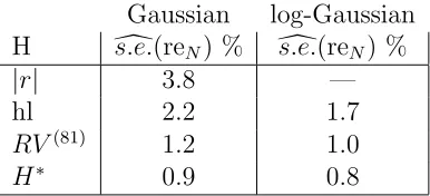
compare the quality of the estimators. Table 1 provides an efficiency factor that expresses the efficiency gain with respect to the standard Garch(1,1) QMLE (as 1/ARE). The proxy
H∗ is constructed in de Vilder and Visser (2007). Moving down from absolute returns toH∗
reveals an efficiency gain by a factor 15 for the Gaussian QMLE. The log-Gaussian QMLE yields an efficiency gain by a factor 20. This means thatestimation of(γ, β)based onlog(H∗)
needs roughly 20 times fewer days of observations than the usual QMLE based on squared
close-to-close returns to obtain the same precision for the parameter estimates. There are
no entries for H = |r| for the log-Gaussian QMLE since these would involve taking the log of zeros. The table reflects the differences in the confidence regions in Figure 1. Notice that in this figure the estimate based on |rn| is situated below and to the left of the other
The log-Gaussian QMLE outperforms the Gaussian QMLE for the proxieshl, RV(81),and
H∗. One possible interpretation is that these proxies are closer to having the distribution of
a lognormal random variable than to the absolute value of a Gaussian random variable. In empirical research it has been found that log realized volatility and the log high-low range may have a distribution that is nearly symmetrical and nearly Gaussian, see for instance Andersen, Bollerslev, Diebold and Ebens (2001), and Alizadeh, Brandt, and Diebold (2002). We apply the Delta method of Section 3.4 to obtain the standard errors of the relative error in the volatility extraction. Table 2 lists these standard errors for the final scale factors
σH,n, n=N = 1001.The first entry, 3.8%, suggests that the interval ˆσH,1001±7.6% encloses
the true σH,1001 with probability 95%. The log-Gaussian QMLE based on H∗ gives a more
than 4 times tighter interval. One should not interpret these percentages as typical for this Garch(1,1) process: they depend on the path of the process before n= 1001.
We also checked what Tables 1 and 2 would look like if they are based on the full sample over the years 1988–2006, n = 1, . . . ,4575, (ignoring possible structural breaks). We briefly mention these results without providing the tables. For the full sample the patterns in both tables are similar to the patterns in Tables 1 and 2, though the efficiency gains in Table 1 become more pronounced: instead of a factor 20 for the log-Gaussian QMLE based on H∗,
we find a gain by a factor more than 40.
Gaussian log-Gaussian
H var(c Z2
H) eff. factor var(log(c ZH2)) eff. factor
|r| 3.34 1 — —
hl 1.41 2.4 0.68 4.9
RV(81) 0.48 7.0 0.25 13.2
H∗ 0.23 14.8 0.17 20.1
Table 1: Empirical QMLE efficiency for the volatility proxies: absolute return, high-low, realized volatility based on 81 five-minute intervals, and H∗. The table reports var(c Z2
H) and var(log(c ZH2)), see Sections 3.1 and 3.2. The numbers are based on residuals of Garch(1,1) estimation of the S&P 500 over 1992–01–01 to 1995–12–31, or 1001 observations. The efficiency factor is the gain with respect to the usual Garch(1,1) QMLE, expressed as 1/ARE, so 2.4=3.34/1.41.
5
Finite-Sample Properties
Gaussian log-Gaussian H ds.e.(reN) % ds.e.(reN) %
|r| 3.8 —
hl 2.2 1.7
RV(81) 1.2 1.0
[image:17.595.196.389.85.173.2]H∗ 0.9 0.8
Table 2: Estimates of the standard error of the relative error in ˆσH,1001. The quantities reported are
100×s.e.(ˆc σH,N)/σˆH,N, see also equation (20). Numbers are based on the same volatility proxies and data as in Table 1.
and Wooldridge (1992), Lumsdaine (1995), Fiorentini, Calzolari, and Panattoni (1996), and Straumann (2005). The simulations in the present paper focus on the difference between the inference based on the close-to-close returns Hn = |rn| and inference by the square root of
realized variance
Hn =RVn(m) =
q
RQVn(m).
To generate the realized variance one has to simulate the process Ψ(·) at (m+ 1) equidistant points in [0,1]. A Brownian motion will not do, since the realized volatility based on 81 intervals then has var(log(Z2
H))≈0.025, which would yield unrealistically precise parameter
estimates, cf. RV(81) in Table 1, which has var(log(Z2
H))≈0.25 where ZH =RV(81)(Ψ).
We consider an intraday diffusion, with an Ornstein-Uhlenbeck process for the log of the diffusion coefficient:
dΨ(u) = exp(Y(u))dB(1)(u), u∈[0,1], (22)
where Y(u) is Ornstein-Uhlenbeck:
dY(u) =−δ(Y(u)−µ)du+σYdB(2)(u). (23)
The Brownian motions B(1) and B(2) are uncorrelated, Ψ(0) = 0, Y(0) =Y
0. We sample Y0
from its stationary distribution. Forµ=−σ2
Y/(2δ), the realized varianceRQV(m)(Ψ) for all
m, as well as the quadratic variation over the unit interval have expectation 1, see Appendix D. Choose
δ= 1
2, σY = 1
4, µ=−
Then the return innovations Zn satisfy
EZ2 = 1, var(Z2)≈2.77.
For the realized volatility we take m = 81 intervals, yielding innovationsZH that satisfy
EZ2
H = 1, var(ZH2)≈0.27, var(log(ZH2))≈0.24. (24)
The simulations below consist of 10000 replications. First generate 10000 sets of 2500 days of realizations of Ψ. For each sequence (Ψn), n = 1, . . . ,2500, we generate the paths (vnτ)
for five different configurations (γ, β),fixing τ = 1. One may now examine the finite-sample properties of the Garch(1,1) QMLE’s (ˆγ,βˆ) for sample lengths N = 250, 500, 1000, 2500.
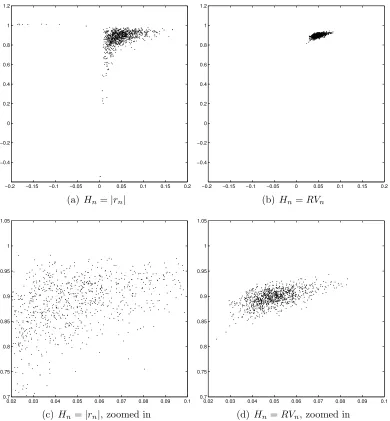
Figure 2 shows the estimates for 1000 of such paths for (γ, β) = (0.05, 0.9) and sample length
N = 1000 days. The left figures are based on absolute returns as a volatility proxy, the right figures are based on the realized volatility RVn(81). The estimates based on RVn(81) are more
concentrated around the true parameter value, and have no outliers.
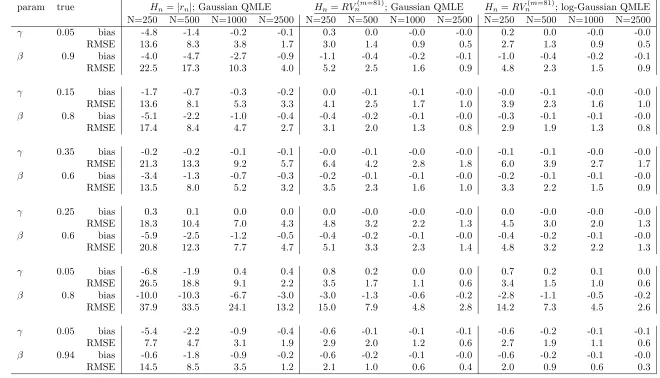
Table 3 provides a more complete overview of the finite-sample properties than Figure 2. The first two rows list 100 × the bias and 100 × the root mean square error (RMSE) of ˆγ
for (τ, γ, β) = (1, 0.05, 0.9). The first four columns in the first row contain the biases for the return based Garch(1,1) QMLE for increasing sample sizes. The next eight columns give this bias using the volatility proxy RVn(81), for the Gaussian and the log-Gaussian QMLE.
While the small-sample biases of ˆγ,βˆtend to be substantial for the return based QMLE, they are moderate to negligible for the realized volatility based QMLE. The asymptotic relative efficiencies with respect to the usual Garch(1,1) QMLE may be deduced from equation (24) and equations (13) and (17). For the square root of realized variance this yields an efficiency factor 2.77/0.27 ≈ 10 for the Gaussian QMLE and efficiency factor 11 for the log-Gaussian QMLE. So the RMSE for Hn = RVn is more than a factor three smaller for
large samples. This factor reflects the difference in RMSE between using returns or realized volatility, for N = 2500. For smaller sample sizes the efficiency gain is larger, suggesting that return based estimation suffers more from small-sample effects. The quality of the parameter estimates using 250 observations of realized volatility resembles using somewhere between 1000–2500 close-to-close returns. As predicted by the asymptotic efficiency factors for RVn computed above (11 versus 10), the log-Gaussian QMLE does slightly better than
−0.2 −0.15 −0.1 −0.05 0 0.05 0.1 0.15 0.2 −0.4
−0.2 0 0.2 0.4 0.6 0.8 1 1.2
(a) Hn=|rn|
−0.2 −0.15 −0.1 −0.05 0 0.05 0.1 0.15 0.2 −0.4
−0.2 0 0.2 0.4 0.6 0.8 1 1.2
(b) Hn =RVn
0.02 0.03 0.04 0.05 0.06 0.07 0.08 0.09 0.1 0.7
0.75 0.8 0.85 0.9 0.95 1 1.05
(c) Hn=|rn|,zoomed in
0.02 0.03 0.04 0.05 0.06 0.07 0.08 0.09 0.1 0.7
0.75 0.8 0.85 0.9 0.95 1 1.05
[image:19.595.97.487.147.568.2](d) Hn =RVn,zoomed in
ˆ
γ,βˆ Sampling Distributions
100×bias, 100×RMSE param true Hn=|rn|; Gaussian QMLE Hn=RV
(m=81)
n ; Gaussian QMLE Hn =RV
(m=81)
n ; log-Gaussian QMLE N=250 N=500 N=1000 N=2500 N=250 N=500 N=1000 N=2500 N=250 N=500 N=1000 N=2500
γ 0.05 bias -4.8 -1.4 -0.2 -0.1 0.3 0.0 -0.0 -0.0 0.2 0.0 -0.0 -0.0
RMSE 13.6 8.3 3.8 1.7 3.0 1.4 0.9 0.5 2.7 1.3 0.9 0.5
β 0.9 bias -4.0 -4.7 -2.7 -0.9 -1.1 -0.4 -0.2 -0.1 -1.0 -0.4 -0.2 -0.1
RMSE 22.5 17.3 10.3 4.0 5.2 2.5 1.6 0.9 4.8 2.3 1.5 0.9
γ 0.15 bias -1.7 -0.7 -0.3 -0.2 0.0 -0.1 -0.1 -0.0 -0.0 -0.1 -0.0 -0.0
RMSE 13.6 8.1 5.3 3.3 4.1 2.5 1.7 1.0 3.9 2.3 1.6 1.0
β 0.8 bias -5.1 -2.2 -1.0 -0.4 -0.4 -0.2 -0.1 -0.0 -0.3 -0.1 -0.1 -0.0
RMSE 17.4 8.4 4.7 2.7 3.1 2.0 1.3 0.8 2.9 1.9 1.3 0.8
γ 0.35 bias -0.2 -0.2 -0.1 -0.1 -0.0 -0.1 -0.0 -0.0 -0.1 -0.1 -0.0 -0.0
RMSE 21.3 13.3 9.2 5.7 6.4 4.2 2.8 1.8 6.0 3.9 2.7 1.7
β 0.6 bias -3.4 -1.3 -0.7 -0.3 -0.2 -0.1 -0.1 -0.0 -0.2 -0.1 -0.1 -0.0
RMSE 13.5 8.0 5.2 3.2 3.5 2.3 1.6 1.0 3.3 2.2 1.5 0.9
γ 0.25 bias 0.3 0.1 0.0 0.0 0.0 -0.0 -0.0 -0.0 0.0 -0.0 -0.0 -0.0
RMSE 18.3 10.4 7.0 4.3 4.8 3.2 2.2 1.3 4.5 3.0 2.0 1.3
β 0.6 bias -5.9 -2.5 -1.2 -0.5 -0.4 -0.2 -0.1 -0.0 -0.4 -0.2 -0.1 -0.0
RMSE 20.8 12.3 7.7 4.7 5.1 3.3 2.3 1.4 4.8 3.2 2.2 1.3
γ 0.05 bias -6.8 -1.9 0.4 0.4 0.8 0.2 0.0 0.0 0.7 0.2 0.1 0.0
RMSE 26.5 18.8 9.1 2.2 3.5 1.7 1.1 0.6 3.4 1.5 1.0 0.6
β 0.8 bias -10.0 -10.3 -6.7 -3.0 -3.0 -1.3 -0.6 -0.2 -2.8 -1.1 -0.5 -0.2 RMSE 37.9 33.5 24.1 13.2 15.0 7.9 4.8 2.8 14.2 7.3 4.5 2.6
γ 0.05 bias -5.4 -2.2 -0.9 -0.4 -0.6 -0.1 -0.1 -0.1 -0.6 -0.2 -0.1 -0.1
RMSE 7.7 4.7 3.1 1.9 2.9 2.0 1.2 0.6 2.7 1.9 1.1 0.6
β 0.94 bias -0.6 -1.8 -0.9 -0.2 -0.6 -0.2 -0.1 -0.0 -0.6 -0.2 -0.1 -0.0
[image:20.842.124.784.81.459.2]RMSE 14.5 8.5 3.5 1.2 2.1 1.0 0.6 0.4 2.0 0.9 0.6 0.3
Table 3: Sampling distributions of Garch(1,1) QMLE, based on 10000 replications. The intraday process Ψn(·) is given by equations (22) and (23) with (δ = 0.5, σY = 0.25, µ=−0.125). All simulations useτ = 1.From top to bottom there are six panels of different parameters (γ, β).For each parameter setting the table gives 100×the bias and 100×the root mean squared error of ˆγand ˆβ, for different lengths of the
6
Conclusions
This paper develops Garch quasi maximum likelihood estimation based on intraday volatility proxies. One may achieve a substantial efficiency gain by using a suitable volatility proxy other than the absolute or squared close-to-close return. The paper starts out from the Garch(1,1) system
rn = vnτ Zn
vn2 = 1 +γr2n−1 +βv2n−1,
and makes use of the extension of the returns rn to the intraday return process Rn(u) =
vnτΨn(u), u ∈ [0,1], where the processes Ψn(·) are iid over different days. The setup
does not make particular assumptions for the process Ψn. One obtains sharp estimators
ˆ
γ, βˆby making use of a suitable volatility proxy H(Rn). Here, H is positive and positively
homogeneous. For the S&P 500 index data the estimated variances of the estimators decrease by a factor 20. The QMLE has the additional advantage that it does not require the usual condition that the conditional fourth moment of the close-to-close returns is finite. The QMLE works provided that the proxy H has a finite conditional fourth moment.
A good parameter estimation for financial processes is important for several reasons. It gives better predictions for future market behaviour. A sharp estimation procedure may also clear up fundamental questions around the stationarity of certain financial processes. Do parameters change over time? Is this change slow or abrupt? We hope that the results in this paper help to find answers to such questions in the future.
The intraday extension employed in this paper and the resulting QML theory apply equally well to other volatility models. It would be interesting to apply the methods of this paper to asymmetric Garch models, or to models where the volatilityvnis driven by statistics
different from the squared return r2
n−1. For instance, from Andersen et al. (2003) we know
that a log-ARFIMA model for realized volatilities fits well. One may expect that realized volatilities could also enhance the latent volatilities vn.We leave this to future research.
7
Acknowledgment
Appendices
A
Data
Our data set is the U.S. Standard & Poor’s 500 stock index future, traded on the Chicago Mercantile Exchange (CME), for the period 1st of January, 1988 until May 31st, 2006. The data were obtained from Nexa Technologies Inc. (www.tickdata.com). The futures trade from 8:30 A.M. until 15:15 P.M. Central Standard Time. Each record in the set contains a timestamp (with one second precision) and a transaction price. The tick size is $0.05 for the first part of the data and $0.10 from 1997–11–01. The data set consists of 4655 trading days. We removed sixty four days for which the closing hour was 12:15 P.M. (early closing hours occur on days before a holiday). Sixteen more days were removed, either because of too late first ticks, too early last ticks, or a suspiciously long intraday no-tick period. These removals leave us with a data set of 4575 days with nearly 14 million price ticks, on average more than 3 thousand price ticks per day, or 7.5 price ticks per minute.
There are four expiration months: March, June, September, and December. We use the most actively-traded contract: we roll to a next expiration as soon as the tick volume for the next expiration is larger than for the current expiration.
Figure 3 gives an impression of the course of volatility over the years 1988–2006. It depicts the cumulative of volatility. The left figure is based on squared daily close-to-close returns, the right one on the daily realized variance based on five-minute returns. The slope in the figure based on realized variance is smaller, since it does not take into account the overnight return. The growth of cumulative volatility is low in certain periods and high in other periods. The years 1992–1995 form a period without clear qualitative changes in the level of volatility. The empirical analysis in Section 4 is based on these four years.
B
Quasi Maximum Likelihood
1988 1990 1992 1994 1996 1998 2000 2002 2004 2006 0
0.05 0.1 0.15 0.2 0.25 0.3 0.35 0.4 0.45 0.5
cumulative volatility
(a) Cumulative ofr2
n
1988 1990 1992 1994 1996 1998 2000 2002 2004 2006 0
0.05 0.1 0.15 0.2 0.25 0.3 0.35 0.4 0.45 0.5
cumulative volatility
[image:23.595.98.491.82.262.2](b) Cumulative ofRQVn
Figure 3: S&P 500 cumulative volatility over the years 1988–2006. Figure (a) estimates cumulative volatility by the sum of squared daily close-to-close returns. Figure (b) shows the cumulative of the daily realized variance,RQVn,based on 81 five-minute returns.
B.1
Principle of QML
The estimation method used in this paper is quasi maximum likelihood (QML). Let us briefly describe the principle of Gaussian quasi maximum likelihood estimation, as discussed in Bollerslev and Wooldridge (1992). Let (yn) be a stationary sequence adapted to the
filtration (Fn). The conditional mean and variance functions µn(θ), hn(θ) are parameterized
by a finite dimensional parameter θ and there is a true value θ0 ∈Θ in the sense that
µn(θ0) =E(yn|Fn−1), hn(θ0) = var(yn|Fn−1), (25)
for all n. The likelihood of the sample (y1, . . . , yN) is a function of θ. The parameter θ may
be estimated by maximizing the Gaussian likelihood, even if the true conditional probability distribution ofynis not Gaussian. The likelihood is constructed then as ifynisN(µn, hn),and
is called quasi-likelihood. Let the residual functionεn(θ) =εn(yn, θ) denote the standardized
yn,
εn(θ) =
yn−µn(θ)
p
hn(θ)
This leads to a log-likelihood
LN(θ) = N
X
n=1
ln(θ), (26)
where, by the Gaussian likelihood,
ln(θ) =−
1
2 [log(2π) + log(hn(θ)) +εn(θ)
2].
Let the QMLE ˆθN denote the maximizer of the log-likelihood. Under regularity (see Appendix
B.2) the QMLE is asymptotically normal,
√
N(ˆθN −θ0) d
→ N(0, V0), N → ∞, (27)
where
V0 =A−01B0A−01. (28)
The matrices A0 and B0 are given by the expected Hessian and the expectation of the outer
product of the scores (which is the covariance matrix of the scores):
(A0)i,j =−E
∂2l 0(θ0)
∂θi∂θj
, (B0)i,j =E s0,i(θ0)s0,j(θ0),
where, using stationarity, the expectation is taken at timen = 0. The scoressn,i(θ) are given
by
sn,i(θ) =
∂ln(θ)
∂θi
= pεn(θ)
hn(θ)
∂µn(θ)
∂θi
+ε
2
n(θ)−1
2hn(θ)
∂hn(θ)
∂θi
.
The expected Hessian A0 may be expressed as
(A0)i,j =E
1
h0(θ0)
∂µ0(θ0)
∂θi
∂µ0(θ0)
∂θj
+ 1
2h2 0(θ0)
∂h0(θ0)
∂θi
∂h0(θ0)
∂θj
.
If the true conditional probability distribution is Gaussian, the QMLE reduces to the Gaus-sian maximum likelihood estimator and the information matrix equality A0 =B0 holds, so
B.2
QML Regularity Conditions
Bollerslev and Wooldridge (1992) provide abstract regularity conditions allowing for addi-tional regressors (xn),and without assuming stationarity for (yn).We restate these conditions
below, assuming stationarity, and leaving out xn. The scores sn are row vectors. Let ¨ln
de-note the Hessian of ln(θ),so ¨ln = ˙sn. We first state the definition of the Uniform Weak Law
of Large Numbers, as given by Wooldridge (1990, Definition A.1). A sequence of random functions qn(yn, θ) satisfies the UWLLN if
sup
θ∈Θ|
N−1
N
X
n=1
qn(yn, θ)−Eqn(yn, θ)| P
→0, N → ∞.
The QML regularity conditions are:
1. Θ is compact, has nonempty interior and θ0 ∈int Θ.
2. The mean and variance functions µn, hn are measurable functions of the data for all
θ ∈Θ,are twice continuously differentiable with respect toθ on int Θ,and the variance is nonsingular (with probability one), for all θ ∈Θ.
3. (a) (ln(θ)) satisfies the UWLLN.
(b) θ0 is the identifiably unique maximizer of El
n(θ).
4. (a) The Hessians (¨ln(θ)) satisfy the UWLLN.
(b) The expected Hessian A0 =E¨ln(θ0) is positive definite.
5. (a) The expected outer productB0 =Es′nsn(θ0) is positive definite.
(b) 1
√
NB
−1/2 0
P
s′
n(θ0) d
→ N(0, Ip), N → ∞.
6. The outer product of the scores (s′
nsn(θ)) satisfies the UWLLN.
B.3
QML Regularity Conditions for Garch(1,1)
The verification of the conditions for asymptotic normality of quasi maximum likelihood given in Appendix B.2, has to be carried out on a case-by-case basis. The Garch(1,1) system (1) and (2) corresponds toyn =rn, µn(θ) = 0, hn(θ) =v2n(γ, β)τ2,with θ= (τ, γ, β).In the case
ˆ
vn(θ).The unobserved volatility is approximated by the volatility recursion, with initialization
ˆ
v2
0 > 0. There are several papers on the Gaussian QMLE for Garch(1,1) including Lee and
Hansen (1994), Lumsdaine (1996), Berkes, Horvath, and Kokoszka (2003), and Francq and Zako¨ıan (2004). The QMLE ˆθN satisfies the asymptotic normality of equation (27) and one
may consistently estimate the covariance matrixV0 by using the empirical counterparts ofA0
and B0; we refer to Straumann and Mikosch (2006) for the following regularity conditions,
see also the monograph of Straumann (2005). The observations y1, . . . , yN are part of a
stationary sequence (yn) that satisfies (cf. (1) and (2))
yn = vnτ Zn (29)
vn2 = 1 +γτ2vn2−1Zn2−1+βv2n−1, (30)
where
1. (Zn) is an iid sequence with EZ2 = 1,
2. τ >0, γ >0, β ∈[0,1),
3. Elog (γ0(τ0)2Z2+β0)<0,
4. Z2 is non-degenerate,
5. EZ4 <∞,
6. P(|Z| ≤z) =o(zµ) as z ↓0,for some µ >0.
Condition (6) is fulfilled if Z has a density that is bounded in a neighbourhood of zero. Straumann and Mikosch (2006) also require EZ = 0 in condition (1) to ensure that yn has
mean zero. As we observe in Section 3.1, the requirement EZ = 0 is not needed, see also Francq and Zako¨ıan (2004). To be precise, one should read condition (2) as: Θ is a compact subset of the space given by condition (2), and θ0 ∈ int Θ. Condition (3) is the usual
condition for strict stationarity and ergodicity of the Garch process. If γ0(τ0)2 +β0 < 1
then condition (3) is fulfilled by Jensen’s inequality, and in addition the process is weakly stationary. Condition (4) is needed for the identifiability of θ.For consistency it suffices that
EZ2 < ∞, but condition (5) is necessary for asymptotic normality of the Gaussian QMLE.
Instead of (Zn) iid in condition (1), Lee and Hansen (1994) use the weaker constraint that
(Zn) is strictly stationary, ergodic. They require that E(Zn4|Fn−1) is uniformly bounded, and
that supnE(log(γ0(τ0)2Z2
C
Proofs
Proof of Theorem 3.1. The proof of Theorem 3.1 in the present paper applies the likelihood
theory of Straumann and Mikosch (2006). The asymptotic normality of the usual Garch(1,1) QMLE follows from Theorem 8.1 of Straumann and Mikosch (2006). The proof of that theorem relies on their more general Theorem 7.1. We extend the assumptions needed to invoke Theorem 8.1 in Straumann and Mikosch, check that this set of assumptions estab-lishes asymptotic normality of the Gaussian QMLE in the present paper, and then remove the redundant assumptions. We collected the conditions for the usual Gaussian QMLE based on close-to-close returns as conditions (1) to (6) in our Appendix B.3. Let us extend these assumptions by duplication: copy the conditions for τ and Z to τH and ZH : assume τH >0
and add to each condition forZ the same condition forZH.We now have a set of (temporary)
conditions (D1) to (D6), concerning both Z and ZH.
Under conditions (D1) to (D4) the usual Garch model satisfies the consistency conditions (C1) to (C4) of Straumann and Mikosch, pp. 2473 (for a verification, see their Section 5.2). Let us first verify that the Gaussian QMLE in the present paper is consistent. LetLH,N(θ) =
PN
n=1lH,n(θ) denote the log-likelihood (modulo a constant), where
lH,n(θ) = −
1
2 log(hn(θ)) +H
2
n/hn(θ)
= −1
2
log(hn(θ)) +
v2
n(γ0, β0)(τH0)2ZH,n2
hn(θ)
,
and hn(θ) = vn2(γ, β)τH2. It is important to note that the innovation ZH,n is independent of
hn(θ) and vn and satisfiesEZH,n2 = 1.The function L(θ) =ElH,0(θ) equals
L(θ) =−1
2E
log(h0(θ)) +
v02(γ0, β0)(τH0)2
h0(θ)
.
One may now follow the proof of Theorem 4.1 of Straumann and Mikosch, pp. 2473 part 1.i, to obtain thatLH,N/N converges toLuniformly. The rest of the proof of Theorem 4.1 needs
no adjustment and shows that the QMLE converges almost surely to (τ0
H, γ0, β0).
replacing X by H, until the second display on pp. 2488, for which we may write
˙
LH,n(θ0) = N
X
n=1
˙
lH,n(θ0) =
1 2
N
X
n=1
˙
hn(θ0)
hn(θ0)
(ZH,n2 −1),
where ˙lH,n(θ0) is a martingale difference sequence since ZH,n is independent of Fn−1 and
EZ2
H,n = 1.Accordingly one may apply the central limit theorem for martingale differences,
assumingEZ4
H <∞.So, an application of Theorem 7.1 to the Gaussian QMLE in the present
paper needs EZ4
H <∞, which is satisfied by (D5).
Under conditions (1) to (6) of Appendix B.3, the standard Garch model satisfies condition (N1) to (N4) of Straumann and Mikosch, see also their Theorem 8.1. For the Gaussian QMLE of the present paper we have to establish (N1) to (N4) under our duplicated conditions (D1) to (D6). The only conditions that are left for reexamination are conditions N3.iii and N3.iv:
E||l˙0||Θ < ∞, and E||¨l0||Θ < ∞. Let us follow the lines of Section 8 of Straumann and
Mikosch. We may write
E||H2
0/h0||νΘ = E||h0(θ0)/h0(θ)||νΘEZH,2ν0.
By (D1), EZ2 <∞, and by (D6):
P(|Z| ≤z) =o(zµ) as z ↓0. So by Lemma 5.1 of Berkes
et al. (2003) one hasE||h0(θ0)/h0(θ)||νΘ<∞, for 0≤ν < 1. Therefore
E||H02/h0||Θν <∞, 0≤ν <1.
One may now follow the arguments of Straumann and Mikosch to establish their conditions N.3.iii and N.3.iv. This establishes the asymptotic normality of the Gaussian QMLE of Theorem 3.1 in the present paper.
Let us finally remove the redundant conditions from (D1) to (D6), and establish conditions (A1) to (A6) of Section 3.1. The assumption EZ4
H <∞and equation (6) already imply that
(ZH,n) is an iid sequence with EZH2 = 1, yielding (A1). One should read condition (2) of
Appendix B.3 as a description of the parameter space. This does not need τ > 0, since we optimizeLH overτH,notτ.Furthermoreτ0 >0 is equivalent toτH0 >0 by equation (7), hence
(A2). Condition (D3) is used for establishing stationarity, ergodicity, and invertibility of (vn).
These properties do not rely on the innovationsZH,n,yielding (A3). Condition (D4) helps to
establish thatvn is uniquely determined byθ, again a property that does not depend onZH,
limit theorem to the derivative of LH,N, which only requires EZH4 <∞, and not EZ4 < ∞,
see the arguments above. Consider assumption (D6): P(|Z| ≤z) =o(zµ) as z ↓0,for some
µ >0.This assumption helps to establish||h0(θ0)/h0(θ)||νΘ <∞,for all 0≤ ν <1,see above.
This does not depend on ZH, hence (A6).
Proof of Lemma 3.2. Differentiation yields ∂σ
2
H,0(θ)
∂τH = 2τHv
2 0(θ),
∂σ2
H,0(θ)
∂γ =τ
2
H ∂v2
0(θ)
∂γ ,and ∂σ2
H,0(θ)
∂β =
τ2
H ∂v2
0(θ)
∂β , so
GH(θ) =E
4 τ2 H 2
τHv20
∂v2 0
∂γ
2
τHv20
∂v2 0
∂β
2
τHv20
∂v2 0 ∂γ 1 v4 0( ∂v2 0
∂γ )2
1 v4 0 ∂v2 0 ∂γ ∂v2 0 ∂β 2
τHv20
∂v2 0 ∂β 1 v4 0 ∂v2 0 ∂γ ∂v2 0 ∂β 1 v4 0( ∂v2 0 ∂β) 2 θ . (31)
The lower right block of the inverse of a matrix
A= A11 A12
A21 A22
!
,
equals C−1 = (A
22−A21A−111A12)−1. So theν = (γ, β) block of G−1 equals the inverse of the
2×2 matrix given by
(C)i,j = cov(
1 v2 0 ∂v2 0 ∂νi , 1 v2 0 ∂v2 0 ∂νj
). (32)
Formula (32) does not depend onH.
On the relative error re(σH,n) in Section 3.4. Lethn(θ) =σH,n2 (θ) = vn2τH2. The derivative of
hn is given by
˙
hn=
2τHvn2 τH2(rn2−1+β
∂v2
n−1
∂γ ) τ
2
H(vn2−1+β
∂v2
n−1
∂β )
.
The Gaussian QMLE ˆθN has asymptotic variance V0 = var(ZH2)G−H1(θ0). The asymptotic
variance (N → ∞) of hn(ˆθN) is given by Vhn = ˙hn(θ
0)V
0h˙n(θ0)′. Partition the matrix G
in (31) into τH and (γ, β) blocks. Using partitioned inverses one finds that the asymptotic
variance of hn (for fixed n) equals
Vhn =cvar(Z
2
H)τH4,
where c is a constant that does not depend on H. The asymptotic variance of σH,n = √
may be obtained by the Delta method using formula (21):
VσH,n = 1 4σ4
H,n(θ0)
Vhn. (33)
One sees that the parameter τH drops out.
D
Realized Variance of Ornstein-Uhlenbeck Log-Volatility
Consider the intraday process Ψ(·) of Section 5. The accompanying volatility process Y(·) satisfies
Y(u) = exp(−δu)Y(0) +µ(1−exp(−δu)) +σY
Z u
s=0
exp(−δ(u−s))dB(2)(s).
Simulation of the processY is straightforward sinceY(u+ ∆)|Y(u) has a normal distribution with mean
exp(−δ∆)Y(u) + (1−exp(−δ∆))µ,
and variance
σ2Y 1
2δ(1−exp(−2δ∆)),
see for instance Glasserman (2003). The processY has a stationary version which is normally distributed with mean µ and variance σ
2
Y
2δ. We sample Y0 from this stationary distribution:
this yields a simple expression for the expectation of the realized quadratic variation using step size ∆. We shall use that the expectation of the squared increment in Ψ equals the expectation of the increment in the quadratic variation. The expected increment in QV
equals
EQV[u, u+ ∆] =
Z t+∆
s=u
Eexp(2Y(s))ds
=
Z u+∆
s=u
Eexp(2Y0)ds
= exp(2µ+ 2σ
2
Y
So, for µ=−σ2
Y/(2δ),the quadratic variation over the unit interval has expectation 1. This
implies that the realized varianceRQV(m) has expectation 1 for allm. We simulate a realized
variance based on m = 81 intervals. Each of those intervals is divided into 10 subintervals using equally spaced grid points. The simulation of the process Y on all grid points is exact. The value of Ψ on each grid point is obtained by Euler discretization.
References
Alizadeh, S., Brandt, M.W. and Diebold, F.X. (2002). Range-based estimation of stochastic volatility models. The Journal of Finance,57, number 3, 1047–1091.
Andersen, T.G. and Bollerslev, T. (1997). Intraday periodicity and volatility persistence in financial markets. Journal of Empirical Finance, 4, 115–158.
Andersen, T.G., Bollerslev, T., Diebold, F.X. and Ebens, H. (2001). The distribution of realized stock return volatility. Journal of Financial Economics, 61, 43–76.
Andersen, T.G., Bollerslev, T., F.X., Diebold and Labys, P. (2003). Modeling and forecasting realized volatility. Econometrica,71, number 2, 579–625.
Barndorff-Nielsen, O.E. and Shephard, N. (2002). Econometric analysis of realized volatility and its use in estimating stochastic volatility models. Journal of the Royal Statistical
Society, SeriesB, 64, number 2, 253–280.
Berkes, I., Horvath, L. and Kokoszka, P. (2003). Garch processes: structure and estimation.
Bernoulli, 9,number 2, 201–227.
Bollerslev, T. and Wooldridge, J.M. (1992). Quasi-maximum likelihood estimation and inference in dynamic models with time-varying covariances. Econometric Reviews, 11,
number 2, 143–172.
de Vilder, R.G. and Visser, M.P. (2007). Volatility proxies for discrete time models. MPRA Working paper no. 4917.
Drost, F.C. and Klaassen, C.A.J. (1997). Efficient estimation in semiparametric Garch models. Journal of Econometrics, 81,193–221.
Engle, R.F. and Gallo, G.M. (2006). A multiple indicators model for volatility using intra-daily data. Journal of Econometrics, 131, number 1-2, 2–27.
Fiorentini, G., Calzolari, G. and Panattoni, L. (1996). Analytic derivatives and the compu-tation of Garch estimates. Journal of Applied Econometrics.
Francq, C. and Zako¨ıan, J-M. (2004). Maximum likelihood estimation of pure GARCH and ARMA-GARCH processes. Bernoulli, 10,number 4, 605–637.
Ghysels, E., Santa-Clara, P. and Valkanov, R. (2006). Predicting volatility: getting the most out of return data sampled at different frequencies. Journal of Econometrics,131,number 1-2, 59–95.
Glasserman, P. (2003). Monte Carlo Methods in Financial Engineering. Applications of Mathematics 53. Springer.
Hillebrand, E. (2005). Neglecting parameter changes in GARCH models. Journal of
Econo-metrics, 129,number 1-2, 121–138.
Lee, S-W and Hansen, B.E. (1994). Asymptotic theory for the garch(1,1) quasi-maximum likelihood estimator. Econometric Theory, 10, 29–52.
Lumsdaine, R.L. (1995). Finite-sample properties of the maximum likelihood estimator in Garch(1,1) and IGarch(1,1) models: A monte carlo investigation. Journal of Business &
Economic Statistics, 13,number 1, 1–10.
Lumsdaine, R.L. (1996). Consistency and asymptotic normality of the quasi-maximum likeli-hood estimator in igarch(1,1) and covariance stationary garch(1,1) models. Econometrica,
64,number 3, 575–596.
Mikosch, T. and Starica, C. (2004). Nonstationarities in Financial Time Series, the Long-Range Dependence, and the IGARCH Effects. The Review of Economics and Statistics,
86,number 1, 378–390.
Straumann, D. (2005). Estimation in Conditionally Heteroscedastic Time Series Models. Lecture Notes in Statistics 181. Springer.
Straumann, D. and T., Mikosch (2006). Quasi-maximum-likelihood estimation in condition-ally heteroscedastic time series: a stochastic recurrence equations approach. The Annals
Wooldridge, J.M. (1990). A unified approach to robust, regression-based specification tests.