Empirically Based Modeling in the Social Sciences and Spurious Stylized Facts

Munich Personal RePEc Archive

Empirically Based Modeling in the Social

Sciences and Spurious Stylized Facts

Bassler, Kevin E. and Gunaratne, Gemunu H. and

McCauley, Joseph L.

University of Houston

17 October 2007

Online at https://mpra.ub.uni-muenchen.de/5813/

Empirically Based Modeling in the Social Sciences

and

Spurious Stylized Facts

Kevin E. Bassler+_{, Gemunu H. Gunaratne}++ _{, and Joseph L.} McCauley

Physics Department University of Houston

Houston, Tx. 77204 [email protected]

+_{Texas Center for Superconductivity} University of Houston

Houston, Texas

++_{Institute of Fundamental Studies} Kandy, Sri Lanka

Abstract

Hurst exponent Hs generated by the using the sliding window technique on a time series plays the same role as Mandelbrot’s Joseph exponent. Mandelbrot originally assumed that the ‘badly behaved second moment of cotton returns is due to fat tails, but that nonconvergent behavior providess instead direct evidence for nonstationary increments.

1. Introduction

The finance and physics literature contains many papers claiming scaling via Hurst exponents on the one hand, and fat tailed distributions on the other. The expectations of Hurst exponent scaling, fat tailed distributions, and exponent universality have played a central in econophysics. The question what are the underlying market dynamics has remained controversial, but we provide strong evidence for a martingale [1], i.e., diffusive dynamics.

This paper explains in more detail our recent foreign exchange (FX) data analysis [2]. The mainl expectations of econophysics, Hurst exponent scaling, universality, and fat tails are not exhibited by FX markets when nonstationary the increments are correctly treated. Correspondingly, we explain why most existing data analysis claiming fat tails and scaling are wrong, including the original paper on reporting fat tails in cotton returns.

The analysis of this paper can be understood as a tale told by two different variables: First, there is what we define [1,2] as the log return

where p(t) is the price of a stock, bond, or foreign exchange at time t, and pc(t) can be understood as ‘value’ [3], the most probable price, the price that locates the peak of the 1-point returns density f1(x,t) at time t. Then, there is what most other theorists (beginning with Osborne) mean by log returns,

x(t,T)=x(t+T)"x(t)=ln p(t+T)/p(t), (2)

but which is clearly an increment of the log return. The log return x(t) is always a ‘good’ variable both in theory and data analysis, but the use of the log increment x(t,T) in data analysis leads to spurious stylized facts, to spurious scaling with exponent Hs=1/2 and spurious fat tails in a wrongly extracted 1-point returns density fs, where the subscript “s” denotes ‘sliding window’. The two variables will yield identical results iff. a data set or model generates stationary increments x(t,T)=x(T). We show correspondingly that the 1-point returns density f₁(x,t) correctly extracted from FX market time series gives evidence neither for scaling with H over a time scale of a day, nor for fat tails. We speculate that stock prices, in contrast, may exhibit fat tails (but not Hurst exponent scaling) over the same time scale. There is no evidence for market universality, and in far from equilibrium dynamics there is no reason to expect universality.

time series while varying t in the increment x(t,T) with T fixed, and in the presence of nonstationary increments this method cannot generate the correct density f₁(x,t). Instead, the method at best generates a spurious density fs(z,t,T) that we will define precisely below. The sliding window technique would be legitimate, would yield f1(z,T) independent of starting time t iff. the increments were stationary, iff. z=x(t,T)=x(T) independent of the starting time t. But the increments in finance data are not stationary [2], and there is no ergodicity in a nonstationary (i.e., far from statistical equilibrium) time series, so that the sliding window method produces ‘significant artifacts’, spurious stylized facts.

Another conclusion is that scaling doesn’t matter anyway [1], scaling gives us no information whatsoever about either the underlying market dynamics or memory. The purpose of this paper is to explain how to analyze random time series without generating spurious stylized facts. Our method and conclusions are not restricted to finance data but have application to the analysis of stocastically generated time series, whether in physics, economics, biology, or elsewhere. We offer a new viewpoint in the theory of stochastic processes and in data analysis. This paper defines the requireents from extracting knowledge of dynamics from empirically generated time series, whether in the social sciences, turbulence, or elsewhere.

2. Hurst exponent scaling

x(t) = tHx(1), (3)

http://en.wikipedia.org/wiki/Hurst_exponent, where the note added Oct., 2007, is ours). Next, we define selfsimilarity in terms of probability densities, which explains what is meant by asserting that x(t)=tH_{x(1) ‘in distribution’.}

The 1-point density f1(x,t) reflects the statistics collected from many different runs of the time evolution of x(t) from a specified initial condition x(to), where x(0)=0 is required for scaling, but cannot describe correlations or the lack of same. Given a dynamical variable A(x,t),the absolute (as opposed to conditional) average of A is

A(t) = A(x, t)f1(x, t)dx "#

# $

. (4)

From (1), the moments of x must obey

x n

(t_{) =} tnH xn_{(1) =} c nt

nH (5)

Combining this with

x

n

(t) = xn

f₁(x,t)dx "

(6)

we obtain

f1(x, t)=t "H

F(u)_{, (7)}

where the scaling variable is u=x/tH _[1,7].

In contrast, the conditional averages <A(x,t)>cond needed in finance require the 2-point density

or, more to the point, the 2-point transition density (conditional probability density) p2(x,t+T:y,t).

If the absolute average of x(t) vanishes, then the variance is simply

" 2

= x2(t) ₌ x2(1) t2H. (9)

This explains what is meant by Hurst exponent scaling, and also specifies what’s meant by asserting that eqn. (1) holds ‘in distribution’. There, ‘in distribution’ refers strictly to the 1-point density, a quantity that tells us nothing about the underlying dynamics.

The vanishing of the absolute average of x does not mean that there’s no conditional trend: in fractional Brownian motion (fBm), e.g., where <x(t)>=x(0)=0 by construction, the conditional average of x does not vanish and depends on t [7], reflecting either a trend or an anti-trend. In a Markov process, scaling requires that the drift rate depends at worst on t (is independent of x) and has been subtracted, that by “x” we really mean the detrended variable x(t)-∫R(s)ds. Markov processes with x-independent drift can be detrended over a definite time scale, but any attempt to detrend fBm is an illusion because the ‘trend’ is due to long time autocorrelations, not to a removable additive drift term [1]. The attempt to detrend a time series x(t) implicitly assumes an underlying martingale M(t) plus drift A(t), x(t)=A(t)+M(t), and fBm is by construction not of that form [1,7].

do not scale, and it’s the transition density p2, or at least the pair correlations, that’s required to give a minimal description of the underlying dynamics1_{. In particular,} scaling, taken alone, implies neither the presence nor absence of autocorrelations in increments/displacements taken over nonoverlapping time intervals. That is, scaling has nothing whatsoever to say about whether a market is effectively efficient (hard to beat), or is easily beatable, in contrast to what at least one of us incorrectly assumed earlier [3,10].

The financial economics literature reflects wrong claims and wrong assumptions about financial time series. In Fama [11], e.g., the claim is made that returns are uncorrelated, <x(t+T)x(t)>=0. The correct statement, explained below, is that both prices and returns are always correlated, <p(t+T)p(t)>≠0, <x(t+T)x(t)>≠0, but increments in returns approximately vanish after a trading time of 10 minutes: <x(t,T)x(t,-T)>≈0 for T≥10 min. of trading [2]. The latter is effectively the efficient market hypothesis: one cannot make money systematically by trading on either simple averages or pair correlations [1]. Note that an assumption of stationary increments, the confusion of x(t,T) with x(T), would lead one wrongly to assert that returns are uncorrelated. Some statisticians and financial economists [12] treat nonstationary time series as if they cold be transformed into stationary ones, but as we show below this is topologically impossible.

3. Stationary vs. nonstationary increments

Stationary processes are often confused with stationary increments in the literature (see [8] for a discussion). Stationary increments are implicitly assumed in data

1

analyses and simulations whenever a sliding window method is used to extract histograms, and the sliding window method is implicitly assumed whenever x(t,T) is treated as the variable in data analysis (see, e.g., [13]). We define stationary and nonstationary increments and exhibit their implications for the question of long time autocorrelations, or complete lack of autocorrelations. We emphasize that the question of stationary increments, not scaling, is central for the existence of long time correlations.

By increments, we mean displacements x(t,T)=x(t+T)-x(t). Stationary increments of a nonstationary process x(t) are defined by [4,5,7]

x(t + T)"x(t) = x(T), (10)

and by nonstationary increments [1,7,15] we mean that the difference

x(t + T)"x(t) # x(T) (11)

depends on both (t,T), not on T alone. The implications of this distinction for data analysis, and for understanding Hurst exponents, are central. Although the correct 1-point density is f1(x,t)=∫dyf2(y,t+T;x,t) by definition, in the nonstationary increment case the density of increments

z=x(t,T) must be obtained from the two-point density via

fs(z,t,T)= $ dxdyf2(y,t+T;x,t)"(z#y+x) (12)

to obtain histograms for the correct 1-point density f1(z,T) from a single long time series.

The efficient market hypothesis (EMH) is sometimes interpreted to mean that the market is impossible to beat [12], that there are no correlations at all (no systematically repeated price/returns patterns) that can be exploited for profit. Real markets are certainly hard to beat. A Markov market satisfies the condition of an impossible to beat market. But because real markets are very hard if not necessarily impossible to beat, models that generate no autocorrelations in increments are a good zeroth order approximation to real markets [1]. In such models, the autocorrelations in increments x(t,T) and x(t,-T) vanish

(x(t1)" x(t1 " T1))(x(t2 + T2)" x(t2)) = 0, (13)

if there is no time interval overlap,

[t

1 " T1,t1]#[t2,t2 + T2] = $, (14)

sense, is impossible to beat, whereas a martingale market looks Markovian to lowest order (at the level of simple averages and pair correlations), but might be systematically beatable at some higher level of insight. This defines precisely what we mean by “lowest order”. It was Mandelbrot who suggested martingales as reflecting the EMH [15], a real market may exhibit memory but that memory will be hard to find and exploit for profit.

Consider a stochastic process x(t) where the increments are uncorrelated. From this condition we easily obtain the autocorrelation function for returns x(t)

x(t)x(s) = (x(t)" x(s))x(s) + x 2

(s) ₌ x2(s) _> 0, (15)

since x(s)-x(to)=x(s), so that <x(s)x(t)>=<x2(s)>=σ2 is simply the variance in x. This is a martingale condition,

x(t+T) cond =x(t), (16)

or

dyyp" 2(y,t+T x,t)=x. (17)

The result has a nice interpretation: since <x(t,T)x(s)>=0 for s≤t<t+T, future ‘gains’ x(t,T) are uncorrelated with all past returns. We interpret an efficient market to mean that thee are no pair correlations that can be exploited for profit. This doesn’t rule out higher order correlations in a martingale.

We next obtain another central result. Combining

(x(t + T)" x(t))

2

= + (x2(t₊ T) ₊ x2(t) _"2 x(t ₊ T)x(t)

with (14), we get

(x(t + T)" x(t)) 2

= x2(t₊ T) _" x2(t) (19)

which depends on both t and T, excepting the rare case where the variance <x2_{(t)> is linear in t. Martingale increments} are uncorrelated and are generally nonstationary. I.e., we must expect nonstationary increments in effectively efficient markets. The variance <x2_{(t)> of a real FX market is not} linear in t, it has instead very complicated variation with time.

Consider next the class of all stochastic processes with stationary increments, x(t,T)=x(T) ‘in distribution’. Here, we begin with

"2 x(t + T)x(t) = (x(t + T)" x(t)) 2

" (x2₍t ₊ T_{) "} x2₍t_{) ,}

(20)

and then using (8) on the right hand side of (18) we obtain

"2 x(t + T)x(t) = (x

2

(T_{) " (}x2₍t₊ T_{) "} x2₍t_{) (21)}

which differs from (13). The increment autocorrelation function is

2 (x(t)

"

x(t

"

T))(x(t

+

T)

"

x(t))

=

x

2

_(2T)

"

2 x

_(T)

(22)

(

x

(

t

)

"

x

(

t

"

T

))(

x

(

t

+

T

)

"

x

(

t

))

=

x

(

T

) (2

"

1)

(23)

characteristic of fBm [5,7]. This autocorrelation vanishes iff. H=1/2, otherwise the autocorrelations are strong for all time scales T. Such fluctuations violate the EMH, especially if H cannot be approximated as H≈1/2. Note that scaling is not the essential point, is in fact irrelevant: stationarity of the increments, reflected in the t-independent pair correlations (21), is the central requirement for long time increment autocorrelations.

Summarizing, the Hurst exponent H tells us nothing whatsoever about autocorrelations in increments, tells us nothing whatsover about the underlying dynamics apart from scaling itself, and tells us nothing whatsoever about the effficiency or lack of same of a market. In the next two sections we will sharpen the distinction by exhibiting both scaling Markov processes and fBm where H≠1/2.

4. Selfsimilar Ito Processes

An Ito process is generated locally by the stochastic diffferential equation (sde)

dx=R(x, t)+ D(x, t)dB(t) (24)

no trend. Finite memory may be present but we will not write the possible memory explicitly. Instead,

The variance can be calculated from the stochastic integral of (24) as " 2 = ds 0 t

# dxf₁(x, s)D(x, s)

$% % #

, (25)

where x(0)=0, so that scaling of the density and the variance imply that the diffusion coefficient scales as well [8]:

D(x, t)=t2H"1D(u), u=x/tH. (26)

Note that scaling of D does not imply scaling of the transition density p₂(x,t+T;x_o,t).

We can also write the mean square fluctuation about an arbitrary point x(t) globally as

(x(t+T)"x(t) 2

= ds t t+T

# dxf₁(x, s)D(x, s)

"$ $

# = x2

(1) ((t+T)2 H

"t2 H ) (27)

and locally for t>>T as

(x(t+T)"x(t)

2

# t2 H"1

D(u)T

. (28)

Both the global and local mean square fluctuations are useful in FX data analysis. In particular, in () the mean square fluctuation scales with T with Hs=1/2.

Ito processes are 1-1 with Fokker-Planck pdes [8,18] so we work with the drift free Fokker-Planck pde

"_p2

"t = 1 2

"2

"x2 (Dp2)

, (29)

where scaling may occur at best only for f₁(x,t)=p₂(x,t:0,0,).

Model 1-point densities that scale with H are easily calculated [8,18,19]. With

f1(x,t)=t "H

F(u);u=x/tH

(30)

and

D(x, t)=t2H"1D(u), u=x/tH (31)

the Fokker-Planck pde (32) yields

2H(uF(u)) "+(D(u)F(u)) ""=0 (32)

which we integrate to obtain

F(u)= C

D(u)e

"2H udu/D(u)# ₍₃₃₎

For H≠1/2 all of these processes generate nonstationary

increments.

D(u)=(1+ u )/2H (34)

Then we get the exponential density

F(u)=Ce"u , (35)

where C is the normalization constant. For FX data a 2-sided exponential density is needed and is easily derived.

5. The Minimal Description of Dynamics

A 1-point density cannot be used to identify the underlying dynamics. Given a point density or a diffusive pde for a 1-point density, we cannot even conclude that we have a diffusive process. The 1-point density for fBm, a nondiffusive process with long time increment autocorrelations, satisfies exactly the same diffusive pde as does a Gaussian Markov process, whereas the transition density for fBm satisfies no pde. A detrended diffusive process has no increment autocorrelations, so that the pde for the transition density is also diffusive (Fokker-Planck). Therefore, the minimal knowledge needed to identify the c of dynamics is either the transition density depending on 2 points, or else the specification of the pair correlations <x(t)x(s)> or increment autocorrelations. Nothing less will suffice.

case where pair correlations determine the process is for Gaussian processes. There, the pair correlations specify the required Gaussian densities of all orders [20].

Here, we cannot determine whether an underlying stochastic process is diffusive, has long time memory like fBm, or arises from correlated noise as in statistical physics near thermal equilibrium without specifying <x(t)x(s)>. Two of these three cases are treated below in the text.

6. Inequivalence of stationary and nonstationary processes

We showed earlier that, incontrast with claims made in many financial math texts, an arbitrary martingale is topologically inequivalent to a Wiener process [1]. By a similar path we can show that nonstationary time series are topologically inequivalnt to stationary ones. By treating time series as if the noise would always be white, this problem has been seriously mishandled in regression analysis [12].

In regression analysis it’s sometimes assumed that a nonstationary time series can be transformed into a stationary one. This is generally impossible. Stationarity is an analog of the notion of “integrability” in nonlinear dynamics [1]. We show next that global transformations from nonstationarity to stationarity are topologically impossible.

Locally seen, every sde is a Wiener process (the noise is always locally whilte): with

dx =R(x,t)dt+ D(x,t)dB (36)

x(t) "xo+R(xo, to)#t+ D(xo, to)#B. (37)

With the transformation y=(x-xo)/(√D(xo,to))δt we get a stationary process: <y2>=1, <y>=0, and the density of y is a stationary Gaussian (see also [12], which goes no further than this). Next, we ask if such a transformation is globally possible. As in nonlinear dynamics or differential geometry, this is an integrability question.

The integrability problem can easily be formulated by using Ito calculus. Starting with the sde for x(t) we ask for a global transformation y=G(x,t) to a Wiener process. From a Wiener process B(t) one can trivially transform to a stationary process B(1)=t-1/2_{B(t). Given the sde}

dy =(

"G

"_t +R

"G

"_x +

1 2

"2

G

"_x2 )dt+

"G

"_x DdB_{, (38)}

the condition for a Wiener process is

"G

"t +R

"G

"x + 1 2

"2 G

"x2 = µ(t),

"G

"x D =c=cons tan t ₍₃₉₎

The required integrability conditions (the conditions that G exists globally) are

"2

G

"x_"t =

"2

G

"t_"x ₍₄₀₎

"G

"t = µ(t)#cR/ D+ 1 4

"D "x /D

3/2

,

"G

"x =c/ D ₍₄₁₎

An easy calculation shows that the only process satisfying global integrability is another Wiener process y=µt+cB. A nonstationary process with D(x,t) depending on x cannot be transformed to a Wiener process! Processes with R and D depending only on t are trivially Wiener by a simple transformation of variables.

One can ask more generally if a nonstationary process can be transformed into an asymptotically stationary process like Ornstein-Uhlenbeck. This can also be formulated as an integrability question, and there is at this stage no general answer. Given some asymptotically stationary process

dy ="#(y)dt+ E(y)dB (42)

with the appropriate condition on γ , the conditions are then

"G

"t +#1R/ D$ 1 4

"D "x /D

3/2

=$%(y),

"G

"x D =E(y) (43)

a priori that an arbitrary nonstationary process can be transformed into a stationary one.

A scaling 1-point density can be transformed into a stationary 1-point density, F(u)=tH_f

1(x,t). However, both the transition density p2 (which does not scale) and the Ito sde [21] shows that the u-process is nonstationary.

7. Time Seris Analysis

One needs many runs of the same identical experiment in order to obtain good histograms/statistics and averages. This means that for data analysis we need different N realizations of the time series x_k(t), k=1,…,N, where for good statistics N>>1. At time t each point in each run provides one point in a histrogram. The average of a dynamical variable A(x,t) is then given by

A(x, t) =

1

N A(xk

k=1 N

" (t),t) ₍₄₄₎

where the N values xk(t) are taken from different runs at the same time t. Suppose that the outcome xm(t) occurs Fm times during the N runs, and denote f_m=F_m/N with

N ₌ F

m m=1

n

" . (45)

Then

A(x, t) = fmA(xm

m=1 n

" (t),t)_{. (46)}

A(x,t) = " dxf1(x,t)A(x,t). (47)

This is the absolute average. In finance, for calculating option prices, e.g., we always want instead the conditional average starting from a specific initial condition (xo,to). This would require histograms for f2(y,t:x,s), whereby p2=f2/f1 could then be constructed. In practice this is hard. What one does instead is to first check the increment autocorrelations. If the increment autocorrelations vanish then we have a martingale. Martingales obey diffusive dynamics. If f1 has been extracted, then the diffusion coefficient D(x,t) can be found by solving the inverse problem in the diffusion pde [10,18], both p2 and f1 satisfy the same pde for Ito processes [16,17]. This requires first that one knows the time dependence of f1. If scaling holds then this is easy, one need only find the Hurst exponent H for the variance. But scaling generally does not hold. FX data are traded 24 hours/day. In that case, when we analyze one market, e.g. the London market, then the we must reset the clock and take an arbitrary time, say 9AM, as the starting time each day [2].

First, if the time series is stationary then the 1-point density and all absolute averages are t-independent [14]. In this case we have the ergodic theorem [20,22],

A(x) =

1

N A(xk(t)

k=1 N

" = _# dxA(x)f₁(x) ₍₄₈₎

where the 1-point density is obtained from the time series from ergodicity: Equally sized regions in the one dimensional phase space x are visited equally frequently, so we can obtain coarsegrain the interval xmin<x<xmax into cells and obtain fk by counting how often xk occurs in the time series. If there is no drift and the motion is bounded (takes place in a box) then f1(x)=constant. But finance markets are nonstationary, are very far from statistical equilirium. The equations that describe finance markets do not even admit statistical equilibrium as a possibility.

Second, if the increments are stationary, x(t+T)=x(t)=x(T), then we can obtain f₁(x,T) from a single ,long time series by sliding a window. We start at a point t, read the value of x at the point t+T, and thereby construct a histogram that yields f1(x,T). In this case the log increment x(t)=lnp(t+T)/p(t)=lnp(T)/p(0) is a ‘good’ variable, and a single long time series yields ‘good statistics’. We may test for stationary increments by breaking the time series up into N ‘runs’ of equal length, and then calculating the mean square fluctuation

(x

2

(t,T) = 1 N xk

2 k=1

N

" (t,T) ₍₄₉₎

The reader is now referred to a discussion in chapter 1 of [10] where it’s implicitly argued that nothing can be discovered unless something is periodic, or is in some sense syetematically repeated, or is invariant (period zero). The repetitiveness in ergodicity (quasiperiodicity) , and with stationary increments x(T) = x(t,T) the 2-point density (but not the 1-point density!) is time translationally invariant.

What can we do if we have a single, long time series and the increments are nonstationary and uncorrelated? In this case we must start by making an ansatz. We assume, e.g., that the traders repeat the same stochastic dynamics each day. This is equivalent to asuming that the same diffusion coefficient D(x,t) describes the trading day after day. So each day is a regarded as a rerun of the same ‘experiment’. One can check this as follows. Calculate the mean square fluctuation <x2_{(t,T)> for one day. Then, calculate the same quantity on} the time scale of a week. If the ansatz is true then the weekly plot of the mean square fluctuation will look like 5 repetitions of the daily plot.

If this fails, then there is no need to write finance or economics texts because there is no empirical basis, or any other bais, for discovering any lawful behavior whatsoever. The same argument applies to other social sciences. We would then be in the situation described by Wigner [11,23] where there may be laws of motion but we would have no way to discover them.

on the globe where AMD is traded (to within taxes and trading costs). This is the analog of rotational invariance in physics. There is no corresponding conservation law (there is no Lagrangian to which one can apply Noether’s Theorem [24]) but there is still the invariance that Wigner told us must be present for the effort to succeed.

8. Spurious Stylized Facts

We begin with ‘the observed stylized facts’ of FX markets as stated by Holmes [25]: (i) asset prices are persistent and have, or are close to having, a unit root and are thus (close to) nonstationary; (ii) asset returns are fairly unpredictable, and typically have little or no autocorrelations; (iii) asset returns have fat tails and exhibit volatility clustering and long memory. Autocorrelations of squared returns and absolute returns are significantly positive, even at high-order lags, and decay slowly; (iv) Trading volume is persistent and there is positive cross-correlation between volatility and volume. These statements reflect a fairly standard set of expectations. Next, we contrast those expected stylized facts with the hard results of our recent FX data analysis [2]. Our analysis is based on 6 years of Euro/dollar exchange rates taken at 1 min. intervals.

0, and autocorrelations in increments are approximately zero after 20 min. of trading, <x(t,T)x(t,-T)>≈0. (iii) We find no evidence for fat tails, and no evidence for Hurst exponent scaling on the time scale of a day. Because of nonstationarity of the increments, a 7 yr. FX time series is far too short (the histograms have too much scatter due to too few points) to indicate what may happen on larger time scales. Although we do not present the proof here, volatility clustering does not indicate ‘long memory’ but is explained as a purely Markovian phenomenon for variable diffusion processes, stochastic processes with diffusion coefficients D(x,t) where the (x,t) dependence is inherently nonseparable [8,18,19]. About point (iv) above, we offer no comment in this paper.

Our main point is: the data analyses used to arrive at the expected stylized facts have all used a technique called ‘sliding windows’ [2]. The aim of this section is to explain that sliding windows produce spurious, results because FX data are nonstationary processes with nonstationary increments. Only one previous FX data analysis [26] that we are aware of showed that sliding windows lead to a spurious Hurst exponent Hs=1/2, and correctly identified the cause as nonstationarity of the increments. We explain that result theoretically below.

produce good statistics because it picks up a lot of data points. But the histograms generated from varying t in the

increments x(t,T) yield f₁(z,T) independently of t iff. the increments are stationary, otherwise the assumption is false.

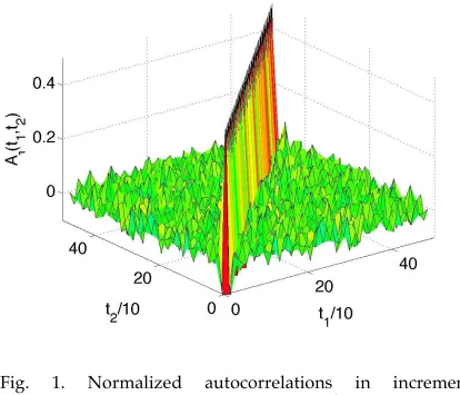
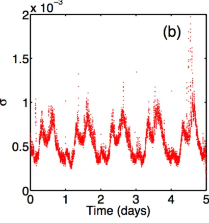
And the assumption is false: first, fig, 1 shows that the increments are uncorrelated after about 10 min. Second, fig. 2a shows that the mean square fluctuation <x2_{(t,T)> with T} fixed at 10 min. depends very strongly on t throughtout the course of a trading day. This means simply that the traders’ noisy behavior is not independent of time of day. Our conclusion is that FX data, taken at 10 min. (or longer) intervals are described by a martingale with nonstationary increments in log returns.

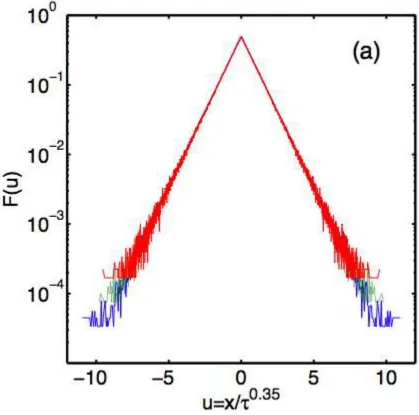
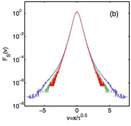
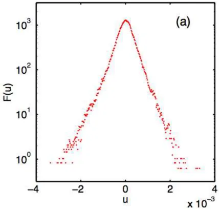
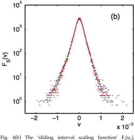
To illustrate how spurious stylized facts are generated by using a sliding window in data analysis, we apply that method to a time series with uncorrelated nonstationary increments, one with no fat tails and with a Hurst exponent H=.35, namely, a time series generated by the exponential density (16) with H=.35 (figure 3a) and linear diffusion (41). The process is Markovian. Fig. 3a was generated by taking 5,000,000 independent runs of the Ito process, each starting from x(0)=0 for T=10, 100, and 1000. The sliding window result is shown as figure 3b. In this case, the sliding windows appear to yield a scale free density Fs(us), u_s=x_s(T)/THs_{, from an empirical average over t that one} cannot formulate theoretically, because for a nonstationary process there is no ergodic theorem. Not only are fat tails generated artificially, but we get a spurious Hurst exponent H_S=1/2 as well. This is the method that has been usedto generate stylized fact’ in nearly all existing finance data analyses.

increments plotted against t in figure 2a, where T=10 min. to insure that there are no autocorrelations in increments (Fig. 1). Second, note that the returns data do not scale with a Hurst exponent H or even with several different Hurst exponents over the course of a trading day (we define a trading day in a 24 hour market by resetting the clock at the same time each morning). Fig. 2b shows that the same stochastic process is repeated on different days of the week, so that we can assume a single, definite intraday stochastic process x(t) in intraday returns. In fig. 2a we see that scaling is observed at best within four disjoint time intervals during the day, and even then with four different Hurst exponents (H<1/2 in three of the intervals, H>1/2 in the other). That is, the intraday stochastic process x(t) generally does not scale and will exhibit a complicated time dependence in the variance <x2_(t)>.

Using the short time approximation T<<t, where t ranges from opening to closing time over a day, we obtain from (27) the mean square fluctuation

x

2

(t,T) " D(x, t)T=t2 H#1

D(u)T

. (50).

With uncorrelated nonstationary increments, in a scaling region we have more generally from (34) that

x

2

(t,T) = (x(t+T)"x(t))2

= x2

(1) [(t+T)2 H

"t2 H

)]

(51)

independent of the details of the diffusion coefficient D(x,t). In most existing data analyses we generally have T/t<<1 when sliding windows are applied to the increments x(T,t), yielding

x 2

(t,T) " x2

(1) 2Ht2 H#1 T

. (52)

Sliding windows then average empirically over t,

x

2

(t,T)

S " x 2

(1) 2H t2 H#1

ST (53)

yielding <x2_(t,T)>

Our exponent sliding window Hs plays the same role for scaling martingales and fBm as does the Joseph exponent J: when there is scaling with H≠1/2 and with no increment autocorrelations then H≠Hs=1/2, whereas for stationary increments with nonlinear variance that scales with H then H=Hs. One need not use R/S analysis [6,28] to look for long time correlations, one need only check the mean square fluctuation <x2_{(t,T)> for lack of t-dependence, for stationary} increments.

9. Are cotton returns fat, or simply nonstationary?

Finally, consider figure 2 in Mandelbrot [29], where fat tails with infinite variance were deduced for cotton returns. He plots what he calls a 2nd _{moment, but is actually a mean} square fluctuation analogous to the mean square fluctuation in our fig. 2a (see also our eqn. (38)). In our notation, the exact quantity analyzed is for a single long time series starting with time to and running through time t is

x2

(s,T) _t

"avg = 1 t"to

x2

(s,T) s=to

t

# (54)

with T fixed at 1 day by using a sliding window. For either a stationary process or for a nonstationary process with finite increments and finite variance this quantity would be expected to ‘converge’ to a constant in probability.

Markets are nonstationary, are very far from statistical equilibrium, and in that case the assumption about the of ergodicity for the empirical time average in eqn. (38) fails. The mean square fluctuation in (54) will not ‘converge’ but will fluctuate eradically if the increments are nonstationary.

The ‘bad behavior’ observed by Mandelbrot has nothing to do with fat tails and is instead direct evidence for nonstationarity of the increments. His figure 2 reminds us of the daily uneveness exhibited by noise traders’ behavior in our fig. 2a. We now explain the basis for our assertion?

For the case of FX data, consider the ensemble average over different trading days. This yields the quantity <x2(t,T)> of our fig. 2a. Next, sum this over different times of day, t-t_o≤24 hrs., as in (54)) to obtain

x2

(s,T)

t"avg

= 1

t"to

x2

(s,T)

s=to

t

# . (55)

As t is increased, according to fig. 2a this quantity should fluctuate wildly due to nonstationarity of the increments. If we would take the quantity (54), without the ensemble average over different trading days, then the fluctuations will be more wild, not less. Mandelbrot’s cotton price fluctuations shown as his fig. 2 are due to nonstationary increments, not fat tails. The cotton variance <x2_{(t)> is both} finite and nonlinear in t, because the increments are nonstationary,

x

2

(t,T) = x2

(t+T) " x2

(t) _{, (56)}

constant ‘in probability’, not wildly fluctuating and ‘nonconvergent’.

Instead of addition of variances, for nonstationary increments we have

"

2

(t+T)="2

(t)+ x2

(t,T) , (57)

Whereas for stationary increments one obtains

"2(t+T)="2(t)+"2(T). (58)

These rules are not like the combination rules for eithe the central limit theorem or for aggregating Levy processes.

Instead of asking ‘is cotton fat?’ it would have been better to ask ‘is cotton a martingale?’ but neither question can be answered by using the sliding window technique implicit in eqn. (54).

Acknowledgement

KEB is supported by the NSF through grant #DMR-0427938. GHG is supported by the NSF through grant #DMS-0607345 and by TLCC. JMC thanks Enrico Scalas and Harry Thomas for very helpful email discussions and is grateful to Giulio Bottazzi for the discussion that led to part 6. This paper is based on the pre-dinner lecture by JMC at the Econophysics Colloquium and Beyond in Ancona, Sept., 27-29, 2007.

References

1. J.L. McCauley, K.E. Bassler, and G.H. Gunaratne,

Martingales, Detranding Data, and the Efficient Market Hypothesis, a A37, 202, 2008.

2. K.E. Bassler, J. L. McCauley, & G.H. Gunaratne,

Nonstationary Increments, Scaling Distributions, and Variable Diffusion Processes in Financial Markets, PNAS 104, 17297, 23 Oct. 2008.

3. J. L. McCauley, K.E. Bassler, & G.H. Gunaratne, On the Analysis of Time Series with Nonstationary Increments in

Handbook of Complexity Research, ed. B. Rosser, 2008.

5.B. Mandelbrot & J. W. van Ness, SIAM Rev. 10, 2, 422,1968.

6. B. Mandelbrot and M.S. Taqqu, 42nd _{Session of the}

International Statistical Institute of Manila, 1, 4-14 Dec. 1979.

7. J. L. McCauley, G. H. Gunaratne, and K. E. Bassler, Hurst Exponents, Markov Processes, and Fractional Brownian Motion, Physica A 369: 343 (2006).

8. K.E. Bassler, G.H. Gunaratne, & J. L. McCauley, Hurst Exponents, Markov Processes, and Nonlinear Diffusion

Equations, Physica A (2006).

9. P. Hänggi, H. Thomas, H. Grabert, and P. Talkner, J. Stat. Phys. 18, 155, 1978.

10. J.L. McCauley, Dynamics of Markets: Econophysics and Finance, Cambridge, Cambridge, 2004.

121. E. Fama, J. Finance 25, 383-417, 1970.

12.See

http://www.xycoon.com/non_stationary_time_series.htm and related papers on regression analysis.

13. T. Di Matteo, T.Aste, & M.M. Dacorogna, Physica A324, 183, 2003.

14. R.L. Stratonovich. Topics in the Theory of Random Noise, Gordon & Breach: N.Y., tr. R. A. Silverman, 1963.

15. B. Mandelbrot, J. Business 36, 420, 1963.

families of Markov processes, and nonlinear Fokker-Planck equations’ by T.D. Frank, Physica A382, 445, 2007.

17. J.L. McCauley, Ito Processes with Finitely Many States of Memory, preprint, 2007.

18. G.H. Gunaratne & J.L. McCauley. Proc. of SPIE conf. on Noise & Fluctuations 2005, 5848,131, 2005.

19. A. L. Alejandro-Quinones, K.E. Bassler, M. Field, J.L. McCauley, M. Nicol, I. Timofeyev, A. Török, and G.H. Gunaratne, Physica 363A, 383, 2006.

20. M.C. Wang & G.E. Uhlenbeck in Selected Papers on Noise and Stochastic Processes, ed. N. Wax, Dover: N.Y., 1954.

21. J. L. McCauley, G.H. Gunaratne, & K.E. Bassler,

Martingale Option Pricing, Physica A380, 351, 2007.

22. A.M. Yaglom & I.M. Yaglom, An introduction to the Theory of Stationary Random Functions. Transl. and ed. by R. A.

Silverman. Prentice-Hall: Englewood Cliffs, N.J., 1962.

23. E.P. Wigner, Symmetries and Reflections. Univ. Indiana: Bloomington,1967.

24. J.L. McCauley, Classical Mechanics: flows, transformations, integrability and chaos. Cambridge Univ. Pr., Cambridge, 1997.

25. C.H. Hommes, PNAS 99, Suppl. 3, 7221, 2002.

27. L. Borland, Phys. Rev. E57, 6634, 1998.

28. J.A. Skjeltorp, Fractal Scaling Behaviour in the Norwegian Stock Market, Masters thesis, Norwegian School of Management, 1996.

29. B. Mandelbrot in P. Cootner, The Random Character of Stock Market Prices, MIT Pr., Cambridge, Mass., 1964.

Figure Captions

nonoverlapping time intervals [t1,t1+T], [t2,t2+T] decay rapidly toward zero for T≥10 min. of trading.

each day as t is varied, exhibiting strongly nonstationary increments. In (a) that we find scaling with H at best in the four disjoint colored regions, and with different values of H in each region.