Open Journal of Applied Sciences, 2014, 4, 23-33
Published Online Februray 2014 in SciRes. http://www.scirp.org/journal/ojapps http://dx.doi.org/10.4236/ojapps.2014.42004
The Calibration of Some Stochastic Volatility
Models Used in Mathematical Finance
Lorella Fatone
1, Francesca Mariani
2, Maria Cristina Recchioni
3, Francesco Zirilli
41Dipartimento di Matematica e Informatica, Università di Camerino, Camerino (MC), Italy 2Dipartimento di Scienze Economiche, Università degli Studi di Verona, Verona, Italy 3Dipartimento di Management, Università Politecnica delle Marche, Ancona, Italy 4Dipartimento di Matematica “G. Castelnuovo”, Università di Roma “La Sapienza”, Roma, Italy
Email: [email protected], [email protected], [email protected], [email protected]
Received 11 November 2013; revised 15 December 2013; accepted 27 December 2013
Copyright © 2014 Lorella Fatone et al. This is an open access article distributed under the Creative Commons Attribution License, which permits unrestricted use, distribution, and reproduction in any medium, provided the original work is properly cited. In accordance of the Creative Commons Attribution License all Copyrights © 2014 are reserved for SCIRP and the owner of the intellectual property Lorella Fatone et al. All Copyright © 2014 are guarded by law and by SCIRP as a guardian.
Abstract
Stochastic volatility models are used in mathematical finance to describe the dynamics of asset prices. In these models, the asset price is modeled as a stochastic process depending on time im- plicitly defined by a stochastic differential Equation. The volatility of the asset price itself is mod- eled as a stochastic process depending on time whose dynamics is described by a stochastic differ- ential Equation. The stochastic differential Equations for the asset price and for the volatility are coupled and together with the necessary initial conditions and correlation assumptions constitute the model. Note that the stochastic volatility is not observable in the financial markets. In order to use these models, for example, to evaluate prices of derivatives on the asset or to forecast asset prices, it is necessary to calibrate them. That is, it is necessary to estimate starting from a set of data of the values of the initial volatility and of the unknown parameters that appear in the asset price/volatility dynamic Equations. These data usually are observations of the asset prices and/or of the prices of derivatives on the asset at some known times. We analyze some stochastic volatili- ty models summarizing merits and weaknesses of each of them. We point out that these models are examples of stochastic state space models and present the main techniques used to calibrate them. A calibration problem for the Heston model is solved using the maximum likelihood me- thod. Some numerical experiments about the calibration of the Heston model involving synthetic and real data are presented.
Keywords
1. Introduction
Stochastic processes, stochastic differential Equations and partial differential Equations are used to describe the dynamics of random phenomena. The study of their relations in mathematical physics begins with the work of
Einstein [1] that establishes the relation between Brownian motion and the heat Equation. More recently random
media and wave propagation in random media have been widely studied [2]. In a random medium, wave motion
is studied as solution of a differential Equation with random coefficients and/or random source terms. The ran- dom coefficients and the random source terms represent the medium and usually are stochastic processes with
known statistical properties. In 1973, Black and Scholes [3] introduced stochastic differential Equations in ma-
thematical finance to model the random behavior of asset prices. The Black and Scholes asset price model can be reduced to Brownian motion with a change of variables. In particular, in the Black and Scholes model, the
option pricing problem can be solved with an explicit formula (i.e. Black and Scholes formula). This model is
elementary and widely used in the financial markets. However,it is known that in several circumstances the as-
set price dynamics model proposed by Black and Scholes in 1973 is inadequate to describe the stock prices ac- tually observed in the financial markets. In particular, the assumption made by Black and Scholes that the asset price volatility is a constant has been criticized. To overcome this difficulty, around 1990, several stochastic vo- latility models of the asset price dynamics had been introduced in the theory and in the practice of mathematical finance. Models of this type are: the Hull and White model, the Stein and Stein model, the Heston model, the SABR model and many others that are not possible to mention individually. In these models the asset price and its volatility at any given time are described by random variables. The time evolution of these random variables is implicitly defined by a system of stochastic differential Equations. This system of stochastic differential Equa- tions equipped with initial conditions and assumptions on the correlations constitutes the model. The stochastic volatility cannot be observed in the financial markets, while the asset price is observable. This means that the stochastic volatility models can be seen as stochastic state space models where the stochastic volatility Equation is the state Equation and the asset price Equation is the observation Equation. The state space models have been
introduced by Kalman in 1960 [4] in the study of guidance and control problems in aerospace engineering and
are widely used. The stochastic volatility models of mathematical finance depend on parameters. Moreover, the initial stochastic volatility, which cannot be observed, must be considered as a parameter. The calibration prob- lem consists in determining the value of these parameters from a set of data. Usually the data are observations of asset prices and/or of prices of options (derivatives) having the asset as underlying at some known times. That is, calibrating a stochastic volatility model means to solve an inverse problem for a stochastic dynamical system. The use of these models in practice is based on the solution of the calibration problem. Several methods have been developed to solve the calibration problem. Let us mention some of them: generalized method of moments, maximum entropy, maximum likelihood, and statistical tests. This review paper introduces the stochastic vola- tility models, explains some of the calibration problems associated to them, illustrates the main calibration me- thods, and considers in detail as an example the problem of calibrating the Heston model with the maximum li- kelihood method using synthetic and real data.
2. Background
In their seminal work [3] Black and Scholes model the dynamics of an asset price through a stochastic differen-
tial Equation. Starting from the idea of Bachelier presented in his doctoral thesis at the École Polytechnique in
Paris [5] of using Brownian motion to model the uncertainty in price behavior Black and Scholes assume that
the asset price evolves according to a geometric Brownian motion with constant drift and volatility. Let t be a
real variable that denotes time and St, t > 0, be a stochastic process that describes the asset price as a function of
time. According to the Black and Scholes model the time dynamics of St, t > 0, is governed by the following
stochastic differential Equation:
dSt =µS ttd +σS W ttd t, >0 (1)
where μ is the constant drift coefficient (i.e. expected return), σ is the constant volatility coefficient of the asset
price St, Wt, t > 0, is a standard Brownian motion and dWt, t > 0, is its stochastic differential.
has become a standard tool to evaluate European call and put options. In 1973 Merton published a paper [6] on pricing theory enhancing the option formula derived by Black and Scholes. For their works Scholes and Merton received the Nobel Prize in Economics in 1997. Unfortunately Black died in 1995. Although the Black and Scholes model is adequate to describe the asset price dynamics in short time intervals, when we consider long time series of option prices the model does not capture some characteristic features of the volatility implied by the observed option prices known as volatility smile and skew. In particular given the observed option prices the volatilities implied by the Black and Scholes formula for options with different strike and maturity are different. This is in contrast with the assumption of the Black and Scholes model that the volatility is a constant. The time series of asset and option prices observed in the financial markets show that the volatility of the asset price is a
non-constant quantity that tends to return over timeto a long-term mean level, that is the behavior of the volatil-
ity can be described satisfactorily by a stochastic mean-reverting process.
3. The Stochastic Volatility Models
The stochastic volatility models try to overcome this inadequacy of the Black and Scholes model assuming that also the volatility is modeled as a stochastic process whose dynamics is described by a stochastic differential Equation. The presence of the volatility term in the Equation that describes the dynamics of the asset price couples the differential Equations for the asset price and for its stochastic volatility generating a system of two stochastic differential Equations. This is the simplest setting of a stochastic volatility model in mathematical finance. These Equations can be interpreted as a model where the asset price propagates in a random medium described by the stochastic volatility. That is stochastic volatility models are somehow similar to the models of propagation in random media used in mathematical physics.
The first authors that have suggested the use of a stochastic volatility model in mathematical finance are Hull
and White in 1987 [7]. The Hull and White model describes the asset price dynamics as follows:
d d d , 0,
d d d , 0.
t t t t t
t t t t
S S t v S W t
v v t v B t
µ
θ ξ
= + >
= + > (2)
where vt, t > 0, denotes the stochastic variance of the asset price St, t > 0, at time t, i.e. the volatility σt, t > 0, is
given by
σ
t = v tt, >0, θ, ξ are, respectively, the drift and the volatility coefficients of the variance vtand μ isthe drift coefficient of the asset price. The quantities θ, ξ, μ are real constants and θ < 0. The stochastic processes
Wt, Bt, t > 0, are standard Brownian motions with correlation coefficient ρ, − < <1 ρ 1 and dWt, dBt, t > 0, are
their stochastic differentials. Note that in (2) the stochastic variance is lognormally distributed and that when θ <
0, we have a zero-reverting process, i.e. the variance tends to return over timeto a long-term zero level. When ρ
= 0 using a second order Taylor expansion with base point ξ = 0 Hull and White derived an explicit formula for
the option prices whose underlying asset price dynamics is described by (2). Moreover the formula for the op-
tion prices was used only when θ is zero. The biggest weakness of this formula is that it is accurate when the va-
riance is almost non-stochastic. In the general case (i.e. ρ≠ 0, θ ≠ 0) the option pricing problem in the Hull and
White model is solved numerically. Note that the assumption ρ = 0 is not supported by observations of asset
prices in the financial markets. In fact the observed prices show that usually ρ is negative.
The Stein and Stein model [8] assumes that:
(
)
d d d , 0,
d d d , 0,
t t t t t
t t t
S S t S W t
t B t
µ σ
σ η θ σ ξ
= + >
= − + > (3)
where μ, η, θ, ξ are real constants such that η > 0 and Wt, Bt, t > 0, are standard Brownian motions with correla- tion ρ, − < <1 ρ 1.
In the Stein and Stein model when η > 0, the stochastic volatility σt, t > 0 follows a mean-reverting
Ornstein-Uhlenbeck process. Note that in this model the volatility can become negative. The Stein and Stein model overcomes the difficulty of the Hull and White model to provide effective option pricing formulae pro- viding a closed-form formula for the prices of the options on a underlying whose price dynamics is described by
(3). This formula is deduced under the assumption ρ = 0.
A very popular stochastic volatility model is the Heston model [9]. The Heston model assumes that the asset
(
)
d d d , 0,
d d d , 0,
t t t t t
t t t t
S S t v S W t
v v t v B t
µ
η θ ξ
= + >
= − + > (4)
where θ is the long-term average of vt, t > 0, η > 0 is the rate of mean-reversion, ξ is the volatility of volatility
coefficient. The quantities μ, θ, η, ξ are real constants, η > 0, and Wt, Bt, t > 0, are standard Brownian motions
with correlation coefficient ρ, − < <1 ρ 1. In the Heston model the variance follows a Cox-Ingersoll-Ross (CIR)
process [10]. The popularity of the Heston model is due to the fact that, when − < <1 ρ 1, it is possible to de-
duce a closed form formula for the price of an European call (put) option whose underlying asset price and its stochastic volatility satisfy Equations (4). The formulae for the option prices are expressed as integrals of expli- citly known integrands. These integrals must be evaluated numerically.
Note that the stochastic volatility models mentioned above assume that the asset price follows the Black and Scholes Equation (1) with stochastic volatility, the difference between them consists in the stochastic process that governs the dynamics of the volatility.
Since the pioneering work of the previous authors many other stochastic volatility models have been intro- duced in mathematical finance. It is not possible to mention all of them. For the convenience of the reader we
just mention one of them: the SABR model [11]. The name SABR is the acronym for “Stochastic Alpha, Beta,
Rho” in fact α, β, ρ are the parameters of the model. The SABR model is widely used to price derivatives on in-
terest rates and currency exchange rates. In the SABR model the time evolution of the asset price and of its sto- chastic volatility satisfy the following system of stochastic differential Equations:
d d , 0,
d d , 0,
t t t t
t t t
S S W t
B t
β
σ
σ ασ
= >
= > (5)
where α and β are real constants such that α > 0, 0≤ ≤β 1 and Wt, Bt, t > 0, are standard Brownian motions
with correlation coefficient ρ, − < <1 ρ 1 . The parameter α is called volatility of volatility coefficient. Note
that the SABR model is a stochastic version of the constant elasticity of variance (CEV) model [12] with skew-
ness parameter β and that it reduces to the CEV model when α = 0. The stochastic volatility models are systems
of stochastic differential Equations and to determine their solution they must be equipped with initial conditions
assigned, for example, at time t = 0.
Unlike the asset price, in the financial markets the volatility cannot be observed. That is the stochastic volatil- ity models are systems of stochastic differential Equations for two dependent variables, one of these variables (the asset price) is observable the other variable (the stochastic volatility or variance) is not observable. If we interpret the stochastic volatility (or variance) as a state variable and the asset price as an observation variable, the stochastic volatility models can be seen as stochastic state space models of a continuous-time dynamic sys- tem. In fact the state (or transition) Equation of the model will be the stochastic differential Equation for the vo- latility (or variance) and the observation (or measurement) Equation of the model will be the Equation for the
asset price. Kalman [4] for a special class of these models has developed a method to estimate the unknown pa-
rameters and the state variable from a time series of values of the observation variable. This technique is known as Kalman filter or linear quadratic estimation (LQE) algorithm. Today state space models and Kalman filters are widely used in science and engineering to study time series of data and to forecast future events based on past data [13].
4. Calibration Methods
Therefore the use of option prices as data for the calibration problem introducesan extra parameter to estimate:
the risk premium parameter. Note that inverse problems for stochastic state space models are widely studied in
many branches of science and engineering. However, the use of option prices as data is a feature that characte- rizes these problem in the context of mathematical finance.
There are several calibration methods, and we discuss briefly the following ones: the generalized method of moments, the maximum entropy method, the maximum likelihood method and the method of statistical tests.
In the generalized method of moments [14] the unknown parameters solution of the calibration problem are
those that minimize the difference between the moments defined by the model of certain variables (i.e. theoreti-
cal moments) and the same moments estimated from the data (i.e. sample moments). In order to use this method
it is necessary to know the analytic expression of the (theoretical) moments or to compute them numerically. Note that the moments of the asset price variable are the natural candidates for the application of the method of
moments. However other choices are possible. For example in [15] the authors starting from the observations of
the asset prices at discrete times apply the generalized method of moments to calibrate square root continuous time stochastic volatility models.
They use as theoretical moments the moments of the integrated volatility conditioned to the observations of the asset price and as sample moments the sample moments of the realized volatility.
The maximum entropy method [16] has his origin in statistical mechanics in the study of the propertiesof
thermodynamicsystems atequilibrium. The idea of the maximum entropy principle, which is the basis of the
homonymous method for the calibration of stochastic volatility models, is to find the values of the unknown pa- rameters of the model as those that maximize the entropy associated to the probability distribution of the asset price and of its stochastic volatility conditioned to the observations. The entropy of a probability distribution
measures the randomness in the probability distribution [17] and in the context of statistical mechanics coincides
with the thermodynamic entropy. Many authors have developed variants of the maximum entropy method, in
particular in [18] the optimal parameters solution of the calibration problem are found as those that minimize the
relative entropy between the probability distribution associated to the model and a reference distribution. The maximum likelihood method determines the unknown parameters of the stochastic volatility model as the parameter values that maximize a likelihood function associated to the data. The likelihood function is a func- tion that measures the probability of obtaining the observed data as a function of the parameter values. The evaluation of the likelihood function usually requires the knowledge of the (joint) probability density function of
the asset price and of its volatility. When the model used is a stochastic volatility model one of the variables (i.e.
the volatility) is not observable so that the use of filtering techniques is necessary to evaluate the likelihood function. Note that given a stochastic volatility model there are several possibilities of defining a meaningful li-
kelihood function. In [19] a closed-form approximation of a likelihood function associated to the Heston model
is derived using a series expansion. The approximate likelihood function is maximized to find the parameters of
the Heston model. In 2006 Bates [20] has found an approximation of a likelihood function associated to expo-
nentially affine stochastic processes. This approximation is built starting from the computation of the inverse Fourier transform of the joint characteristic function of the asset price and its stochastic volatility on the ob- served asset prices. The parameters estimated maximizing the likelihood function are used to forecast the un-
known volatility values. In [21] the joint probability density function of the Heston model conditioned to the
observations is obtained as solution of a sequence of initial value problems for the Fokker-Planck Equation of
the model (i.e. as solution of the Kushner Equation). The likelihood function of the parameters can be expressed
through integrals of this transition probability density function. The main feature that makes the calibration
problem studied in [21] interesting is the use as data of observations of asset prices and of option prices. The use
of this set of data guarantees that the parameters obtained maximizing the likelihood function determine a good match between theoretical option prices and option prices observed in the past and produce satisfactory forecast values of asset and option prices.
Note that the maximum likelihood method is statistically more efficient than the generalized method of mo- ments when this last method is applied using a finite number of moments. In fact the probability density function used in the likelihood function contains more “information” about the model than the “information” contained in a finite number of moments of a variable of the model. However when the evaluation of the likelihood function is difficult or computationally expensive the generalized method of moments can be a valid alternative to the maximum likelihood method.
studied but do not associate a statistical significance level to them. The use of statistical hypothesis testing can overcome this weakness of the previous methods. In this case, the null hypothesis of a statistical test states that the values of the model parameters are equal to the values estimated with one of the methods mentioned pre- viously. Recall that the significance level is the maximum probability of rejecting the null hypothesis when the null hypothesis is true. Starting from the data sample available of the observed asset and/or option prices, the statistical test technique can be used to test the null hypothesis with a given statistical significance level. The idea of using statistical tests to solve calibration problems for stochastic dynamical systems is a very natural one.
In [22] a statistical test procedure to calibrate the Black and Scholes model is presented. The procedure makes
use of elementary statistical tests, that is: the Student’s T and the χ2 tests [23]. The data used to calibrate the
model are the observations on a discrete set of time values of the asset price. Note that when the asset price dy-
namics follows the Black and Scholes model the asset price log-return increments (i.e. the difference between
the asset price log-returns evaluated at different times) obtained when the observation times are equally spaced time values are independent identically distributed Gaussian random variables. This implies that the calibration can be done using the elementary statistical tests already mentioned. In more general contexts when stochastic
volatility models are considered it is necessary to build ad hoc statistical tests. For example in [24] two statistical
tests to calibrate the normal SABR model (with statistical significance level) in correspondence of two different set of data are presented. These statistical tests are based on some new formulae for the moments of the normal SABR model variables and make use of numerical methods.
For the convenience of the reader Table 1 summarizes the calibration methods discussed in this Section and
their properties.
5. An Example: The Calibration of the Heston Model
Let us consider the problem of calibrating the Heston model using the maximum likelihood method. As data of the calibration problem we use a time series of asset and option prices. This problem is an example of calibra- tion of a stochastic volatility model and its solution shows the concrete possibilities of the calibration methods
discussed in Section 4. A similar problem has been studied in [21].
Let us begin completing the Heston model dynamic Equation (4) with the following initial conditions:
,
,
o o o o
S
=
S v
=
v
(6)where
S v
o,
o are given random variables. We assume thatS v
o,
o are concentrated in a point with probabilityone, for simplicity, we identify
S v
o,
o with the points where they are concentrated and we assumeS v
o,
o>
0
.Table 1.Summary of calibration methods and of their properties.
Calibration method Foundation of the method Comment
1 Generalized method of moments
The unknown parameters are obtained minimizing the difference between the moments defined by the model of some random variable and the same moments estimated from the data.
This is the most popular calibration method. Option prices can be seen as moments of random variables. In this case the calibration can be reduced to the least squares fit of theoretical and observed option prices.
2 Maximum Entropy
The unknown parameters are obtained maximizing the entropy of the probability distribution of the asset price and of its stochastic volatility conditioned to the observations. The entropy is a measure of the randomness of a probability distribution.
This method is based on ideas taken from statistical mechanics. Both option prices and asset prices can be used as data. The entropy function can be substituted with an approximate entropy function to save computation.
3 Maximum Likelihood
The unknown parameters are obtained maximizing a likelihood function associated to the data. The likelihood function measures the probability of obtaining the observed data as a function of the parameter values.
Both option prices and asset prices can be used as data. The method exploits the fact that the joint probability distribution of the state variables of the models considered admits a simple integral representation formula.
4 Statistical Tests
The unknown parameters are determined using statistical hypothesis testing. Ad hoc statistical tests are developed to exploit the available data.
Recall that in the financial markets the initial asset price
S
o can be observed while the initial stochastic va-riance vo cannot be observed and must be regarded as a parameter of the model. This means that the Heston
model parameters that must be evaluated from the data in the calibration problem are:
, , , , ,vo
µ η θ ξ ρ . When we consider option prices as data of the calibration problem to the previous parameters
we must add the risk premium parameter λ. In fact the option prices are evaluated with respect to the risk neutral
measure. This is the probability measure associated to the Heston model where η and θ are substituted respec-
tively with η η λ θ, ηθ
η λ
∗= + ∗ =
+ . Let
7
R be the seven dimensional real Euclidean space, the unknown of the
calibration problem is the vector
(
, , , , , ,)
T 7o
v R
µ η θ ξ ρ λ
Θ = ∈ where T denotes the transpose operator. Ele-
mentary considerations suggest that Θ must belong to the following set:
(
)
T 72 2
, , , , , o, R 0, 0, 0, 1, 1 1, o 0, .
M µ η θ ξ ρ v λ η ξ θ ηθ ρ v λ η
ξ
= Θ = ∈ > > > ≥ − ≤ ≤ > > −
(7)
The condition 2ηθ2 1
ξ ≥ is imposed in order to guarantee that when vo >0 with probability one from Equa-
tions (4) follows that vt is positive with probability one for t>0.
The data of the calibration problem studied are:
1) The observation times 0= < < <t0 t1 t2 < < +∞tn , 2) The observed asset price
S
i at time t=ti, 0,1,i= , ,n3) The observed option price
C
i at time t=ti, 0,1,i= , .nThe option prices are the prices of a European call option on the asset whose price is described by the Heston
model with (known) maturity time T >tn and strike price E>0.
We assume that the observation times and the observed asset prices are not affected by observation errors and
that the asset prices are described by the Heston model, while for i=1, 2,,n the i-th observed option price
when compared to the option price of the Heston model is affected by an additive observation error that we as-
sume to be normally distributed with mean zero and known variance φi.
Let
p S v t S v t
(
, , , , ,
′ ′ ′
)
, , , , , ,
S S v v t t
′
′ ′
>
0,
t t
− ≥
′
0,
be the joint probability density function of the stochastic processes implicitely defined by (4), (6), that is letp S v t S v t
(
, , , , ,
′ ′ ′
)
be the probability density function of having St =S v, t =v given the fact that we have St′ =S v′, t′ =v t′, > ≥t′ 0.Moreover letC S v t E T
(
, , , , ,
Θ
)
bethe price at time t when we have St =S v, t =v in the Heston model of parameters Θ of a European call op-
tion with maturity time T >t and strike price E. In the theoretical option price
C S v t E T
(
, , , , ,
Θ
)
we use asdiscount factor μ instead of the risk free interest rate r (i.e. we assume µ =r). This choice simplifies a little bit
the calibration problem. The probability density function p and the call option price C can be written as one di-
mensional integrals of known integrand functions (see, for example [21]). To keep the exposition simple we
omit these formulae.
In the formulation of the calibration problem that follows we use the joint probability density function of the variables S v tt, ,t >0, of the Heston model conditioned to the observations
S C
i,
i made at the times ti suchthat ti<t i, =0,1,,n. This probability density function is a piecewise solution of the forward Kolmogorov
Equation associated to the Heston model. That is the transition probability density function conditioned to the
observations between two consecutive observation times t ti,i+1,i=0,1,, ,n (we define tn+1= +∞) is the solu-
tion of the forward Kolmogorov Equation that satisfies a suitable initial condition at time t=t ii, =0,1,,n.
The initial condition imposed at time t=ti depends from the observations made up to time t ii, =0,1,, ,n
and on the assumptions made about the observation errors (see [21]). For i=0,1,,n let p S v ti
(
, , Θ)
be thejoint probability density function conditioned to the observations made up to time t when ti< ≤t ti+1. The func-
tions p ii, =0,1,, ,n can be expressed using integral representation formulae involving the transition proba-
bility function p (see [21]). To keep the exposition simple we omit these formulae here.
Let us define the likelihood function
F
( )
Θ Θ ∈
,
M
, used in the formulation the calibration problem, that is:( )
1(
1 1) (
1 1 1)
0(
0 0) (
1 0 0)
0
log d , , , , log d , , , , ,
n
i i i i i
i o o
F v p S v t π S v t v p S v t π S v t
+∞ +∞
−
+ + + +
=
Θ = Θ Θ + Θ ⋅ Θ
where
(
)
2(
( ))
21
, , , , , 2
1
1
, , e , 0,1, ,
2π
i i i i
C C S v t E T
i i
i
S v t φ i n
π
φ
− − Θ
Θ = =
. (9)
It is easy to see that the choices of Θ ∈M that make big the function
F
( )
Θ
make big the probability ofdoing the observations
S C
i,
i actually done at time t=t ii, =0,1,,n. This fact justifies the name likelihoodfunction given to the function
F
( )
Θ Θ ∈
,
M
, defined in (8), (9). Note that the choice of the function( )
,
F
Θ Θ ∈
M
, made in (8), (9) is only one possible choice of likelihood function, there are many other ways of defining legitimate likelihood functions.The calibration problem for the Heston model is formulated as follows:
( )
max
F
Θ Θ∈
.
M
(10)This is a constrained optimization problem that must be solved numerically. The objective function of the op-
timization problem
F
( )
Θ Θ ∈
,
M
, contains several integrals that must be evaluated numerically. That is in thenumerical solution of problem (10) the function evaluation can be computationally “expansive”. However since the numerical evaluation of integrals is highly parallelizable when needed parallel computing can be easily used
to speed up the evaluation of the function
F
( )
Θ Θ ∈
,
M
. The constraints contained in M are very simple andare easy to handle numerically. In the numerical experience presented below we solve the calibration problem (10) using a variable metric steepest ascent algorithm.
Let us present two numerical experiments using synthetic and real data.
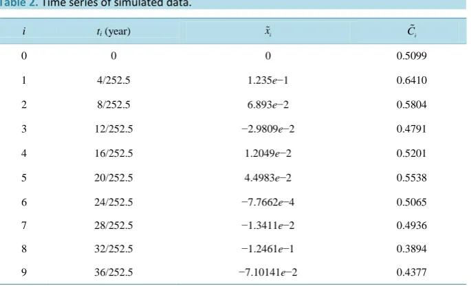
Experiment 1: Calibration of the Heston model using synthetic data. We consider a “year” made of 252.5
trading days, a temporal interval of 36 consecutive trading days and n = 9 observation times in this time period.
We choose t0 =0, and ti =ti−1+ ∆, i=1, 2,, 9, where
4 252.5
∆ = . The vector
Θ
used to generate onetrajectory of the Heston model is:
(
)
(
)
T
T , , , , , ,
0.026, 5.94, 0.306, 0.01159, 0.576, 0.5, 0 .
o
v
µ γ ε θ ρ λ
Θ = = Θ
= −
We have chosen
S
o=
1,
φ
i=
10 ,
−4 i=0,1,, 9. In Table 1 we have defined log i, 0,1, , 9,i
o
S
x i
S
= =
and
[image:8.595.128.471.515.723.2]the notation eX means 10X. Table 2shows the data generated.
Table 2. Time series of simulated data.
i ti (year) xi Ci
0 0 0 0.5099
1 4/252.5 1.235e−1 0.6410
2 8/252.5 6.893e−2 0.5804
3 12/252.5 −2.9809e−2 0.4791
4 16/252.5 1.2049e−2 0.5201
5 20/252.5 4.4983e−2 0.5538
6 24/252.5 −7.7662e−4 0.5065
7 28/252.5 −1.3411e−2 0.4936
8 32/252.5 −1.2461e−1 0.3894
We have F
( )
Θ ≅ 43.15. The initial guess of the optimization method is chosen equal to(
)
0
0.5, 9.22, 0.15, 0.0067, 0.634, 0.3, 0.01 M
Θ = − ∈ . We have Θ − Θ 0 Θ ≈ 0.398,F
( )
Θ = −0 979.1. LetΘ
*be the solution of the calibration problem (10) obtained using the variable metric steepest ascent algorithm, we
have F
( )
Θ =* 43.17 and Θ − Θ * Θ ≈ 0.041.Experiment 2: Analysis of the S & P 500 index. We analyze the daily closing values of the US S&P 500 in-dex and the corresponding bid prices of a European call option on the US S&P 500 inin-dex with maturity date De-
cember 16, 2005 and strike price E = 1200 during the period of about four months going from January 3, 2005 to
May 11, 2005. Due to the number of data actually available in 2005 the time unit is a year made of 253 trading
days. We choose as time t = 0 the day January 3, 2005. We consider 81 windows of 10 consecutive daily obser-
vation times. In particular the observation times are chosen as
t
i j,= +
(
i
j
)
253, 0,1,
i
=
,9,
j
=
0,1,
,80,
thatis in each window we consider daily observations and when we move from a window to the next one we discard the observations made in the first day of the window and we add the next daily observations as last observations to build the new window. The calibration problems procedure, applied to the eighty-one windows considered
provides eighty-one values of the parameter vector Θ of the Heston model. The parameter vectors obtained
from the calibration problems are substantially independent from the data window considered. Finally for
0,1, ,80
j= we use the parameter vector obtained as solution of the calibration problem using the data of the
j-th window to forecast using a filtration method (see [21]) the value of the S&P 500 index and the bid price of
the option the day next to the last observation time of the j-th window. In the eighty-one calibration and fore-
casting problems solved the mean relative error made in the forecasts of the next day S&P 500 index value and option bid price are 0.0063 and 0.0785 respectively.
From the results obtained in Experiment 1 and 2 we can conclude that the validity of the Heston model to in- terpret financial data and the quality of the calibration procedure used are confirmed.
6. Future Research Directions
The stochastic volatility models described in the previous sections can be generalized in many different ways. For example multiscale versions of stochastic volatility models are used in finance to model commodity prices or to evaluate insurance premia. These multiscale models introduce one or more extra stochastic volatility terms in the model. The multiscale version of a model usually increases the number of parameters to estimate making the calibration problem more difficult and more demanding computationally than the calibration problem for the original model. In order to overcome this difficulty it is necessary to develop ad-hoc techniques to simplify the
computation or it is possible to make use of parallel computing. In [25] and in [26], independently, the authors
introduce a multiscale stochastic volatility model that generalizes the Heston model. In the multiscale Heston
model two stochastic volatilities are considered. In [26] an extension of the maximum likelihood method has
been used to calibrate the multiscale Heston model. This calibration is based on the reduction of the dimensio- nality of the integrals that must be computed to evaluate the likelihood function. This reduction of the dimen- sionality of the integrals is obtained computing analytically some of the integrals that appear in the likelihood function. On the other hand in more general situations parallel computing and GPU computing can be used to speed up the evaluation of the likelihood function.
Note that the calibration methods described in the previous section have been applied only to special classes
of stochastic volatility models. For example in [20] and in [21] the authors limit themselves to the calibration of
exponentially affine stochastic volatility models because for these models there exists an explicit formula (in- volving integrals) for the joint characteristic function of asset price and its stochastic volatility. It should be in- teresting and useful to apply the calibration methods to the study of more general classes of models.
Finally cross fertilization between different research areas is possible. In fact, for example, the methods used to solve inverse problems for state space models outside mathematical finance, such as particle filtering, can be
transferred in financial mathematics and used to calibrate stochastic volatility models [27].
7. Conclusion
methods find the unknown parameters of the model as solution of optimization problems and differ in the choice of the objective function of the optimization problem considered. The method that uses statistical tests is the on- ly one that associates a statistical significance to the solution found. However, the choice of the hypothesis to be tested in the solution of the calibration problem may be difficult when models with several parameters (five, six parameters or more) are employed. A way to overcome this difficulty consists in using a different calibration
method (i.e.: generalized method of moments, maximum entropy, …) to determine the solution of the calibration
problem and in using the solution found to formulate the hypothesis to be tested. To this hypothesis is given a statistical significance using the statistical test method. We can conclude that the calibration problems for the stochastic volatility models developed in the nineties have been solved satisfactorily. The dramatic change of financial markets and of computing technologies announces the development of new, more sophisticated, sto- chastic volatility models whose calibration will pose new challenges. We expect that new problems and ideas will arise from considering these new models and the specific features that derive from their origin in finance.
References
[1] Einstein, A. (1905) Über die von der molekularkinetischen theorie der Wärme geforderte Bewegung von in ruhenden Flüssigkeiten suspendierten Teilchen. Annalen der Physik, 322, 549-560. http://dx.doi.org/10.1002/andp.19053220806
[2] Keller, J.B. (1964) Wave propagation in random media. Proceedings of Symposia in Applied Mathematics, 13, 227- 246.
[3] Black, F. and Scholes, M. (1973) The pricing of options and corporate liabilities. Journal of Political Economy, 81, 637-659. http://dx.doi.org/10.1086/260062
[4] Kalman, R.E. (1960) A new approach to linear filtering and prediction problems. Journal of Basic Engineering- Transactions of the ASME, Series D, 85, 35-45. http://dx.doi.org/10.1115/1.3662552
[5] Bachelier, L. (1900) Théorie de la speculation. Annales Scientifiques de l’École Normale Supérieure, 3, 21-86.
[6] Merton, R.C. (1973) Theory of rational option pricing. Bell Journal of Economics and Management Science, 4, 141- 183. http://dx.doi.org/10.2307/3003143
[7] Hull, J. and White, A. (1987) The pricing of options on assets with stochastic volatilities. Journal of Finance, 42, 281- 300. http://dx.doi.org/10.1111/j.1540-6261.1987.tb02568.x
[8] Stein, E.M. and Stein, J.C. (1991) Stock price distribution with stochastic volatility: An analytic approach. Review of Financial Studies, 4,727-752. http://dx.doi.org/10.1093/rfs/4.4.727
[9] Heston, S.L. (1993) A closed-form solution for options with stochastic volatility with applications to bond and curren- cy options. The Review of Financial Studies, 6, 327-343. http://dx.doi.org/10.1093/rfs/6.2.327
[10] Cox, J.C., Ingersoll, J.E. and Ross, S.A. (1985) A theory of the term structure of interest rates. Econometrica, 53, 385- 407. http://dx.doi.org/10.2307/1911242
[11] Hagan, P.S., Kumar, D., Lesniewski, A.D. and Woodward, E. (2002) Managing smile risk. Wilmott Magazine, 2002, 84-108. http://www.wilmott.com/pdfs/021118_smile.pdf
[12] Cox, J. (1975) Notes on option pricing I: Constant elasticity of diffusions. Unpublished Draft, Stanford University. [13] Harvey, A.C., Koopman, S.J. and Shephard, N. (2004) State space and unobserved component models: Theory and ap-
plications. Cambridge University Press, Cambridge.
[14] Hansen, L.P. (1982) Large sample properties of generalized method of moments estimators. Ecometrica, 50, 1029- 1054.
[15] Bollerslev, T. and Zhou, H. (2002) Estimating stochastic volatility diffusion using conditional moments of integrated volatility. Journal of Econometrics, 109, 33-65. http://dx.doi.org/10.1016/S0304-4076(01)00141-5
[16] Jaynes, E.T. (1957) Information theory and statistical mechanics. Physical Review, 106, 620-630.
http://dx.doi.org/10.1103/PhysRev.106.620
[17] Shannon, C.E. (1948) A mathematical theory of communication. Bell System Technical Journal, 27, 379-423.
http://dx.doi.org/10.1002/j.1538-7305.1948.tb01338.x
[18] Avellaneda, M. (1998) Minimum-relative-entropy calibration of asset pricing models. International Journal of Theo- retical and Applied Finance, 1, 447-472. http://dx.doi.org/10.1142/S0219024998000242
[19] Ait-Sahalia, Y. and Kimmel, R. (2007) Maximum likelihood estimation of stochastic volatility models. Journal of Fi- nancial Economics, 83, 413-452. http://dx.doi.org/10.1016/j.jfineco.2005.10.006
[21] Mariani, F., Pacelli, G. and Zirilli, F. (2008) Maximum likelihood estimation of the Heston stochastic volatility model using asset and option prices: An application of nonlinear filtering theory. Optimization Letters, 2, 177-222.
http://dx.doi.org/10.1007/s11590-007-0052-7
[22] Fatone, L., Mariani, F., Recchioni, M.C. and Zirilli, F. (2012) The use of statistical tests to calibrate the Black-Scholes asset dynamics model applied to pricing options with uncertain volatility. Journal of Probability and Statistics, 2012, Article ID: 931609.
[23] Johnson, R.A. and Bhattacharyya, G.K. (2006) Statistics: Principles and methods. 5th Edition, John Wiley & Sons, New York.
[24] Fatone, L., Mariani, F., Recchioni, M.C. and Zirilli, F. (2013) The use of statistical tests to calibrate the normal SABR model. Journal of Inverse and Ill-Posed Problems, 21, 59-84. http://dx.doi.org/10.1515/jip-2012-0093
[25] Christoffersen, P., Heston, S. and Jacobs, K. (2009) The shape and term structure of the index option smirk: Why mul- tifactor stochastic volatility models work so well. Management Science, 55, 1914-1932.
http://dx.doi.org/10.1287/mnsc.1090.1065
[26] Fatone, L., Mariani, F., Recchioni, M.C. and Zirilli, F. (2009) An explicitly solvable multi-scale stochastic volatility model: Option pricing and calibration problems. Journal of Futures Markets, 29, 862-893.
http://dx.doi.org/10.1002/fut.20390