Rainfall Runoff Modeling using Multiple Linear Regression Technique

Rainfall-Runoff Modeling using Multiple Linear

Regression Technique

Lateef Ahmad Dar

Deptt.of Civil Engineering, National Institute of Technology Srinagar, J&K, India.

Abstract: In this paper MLR model was developed to model the rainfall-runoff process. The main objective of this study is to prove that MLR can be successfully used as R-R models. It is for this reason that various MLR models were developed and tested on data sets for the river Jhelum catchment (J&K, India) and later their performance was checked by different statistical parameters like coefficient of determination R2 and root mean squared error (RMSE).

Keywords: Rainfall, Runoff, Modeling, Multiple Linear Regression.

I. INTRODUCTION

Hydrological models are important and necessary tools for water and environmental resources management. Demands from society on the predictive capabilities of such models are becoming higher and higher, leading to the need of enhancing existing models and even of developing new theories. Existing hydrological models can be classified into three types, namely, 1) empirical models (black-box models); 2) conceptual models; and 3) physically based models. To address the question of how land use change and climate change affect hydrological (e.g. floods) and environmental (e.g. water quality) functioning, the model needs to contain an adequate description of the dominant physical processes. Following the blueprint proposed by Freeze and Harlan (1969), a number of distributed and physically based models have been developed, among which are the well-known SHE (Abbott et al., 1986a, b), MIKE SHE (Refsgaard and Storm, 1995), IHDM (Beven et al., 1987; Calver and Wood, 1995), and THALES (Grayson et al., 1992a) models. These models are able to produce variations in state-variables over space and time, and representations of internal flow processes. It is assumed that the parameter values in the equations of such models can be obtained from measurements as long as the models are used at the appropriate scale. Physically- based distributed models particularly aim at predicting the effects of land use change. However, considerable debate on both the advantages and disadvantages of such models has arisen along with research and applications of those models (see, e.g. Beven 1989, 1996a, b, 2002; Grayson et al., 1992b; Refsgaard et al., 1996; O’Connell and Todini, 1996). In general, such models are very data-intensive and time- consuming when applied in a fully distributed manner. In applications, the model scale is generally much larger than the scale of parameter measurements. Therefore, “effective” parameter values have to be adopted in model applications and thus calibration becomes inevitable for physically based models. This leads to the difficulty of parameter identification and the equifinality problem (Beven, 1993, 1996c; Savenije, 2001).Conceptual models form by far the largest group of hydro-logical models that have been developed by the hydrological community and which are most often applied in operational practice. Among those are SAC-SMA (Burnash et al., 1973; Burnash, 1995), HBV (Bergstrom and Forsman, 1973; Bergstrom, 1995), and LASCAM (Sivapalan et al., 1996).Most conceptual models are spatially lumped, neglecting thespatial variability of the state variables and parameters. To improve the potential for making use of spatially distributed data, some lumped conceptual models have been extended to be distributed or semi-distributed. Examples are the HBV-96model (Lindstrom et al., 1997), TOPMODEL (Beven, 1995) and the ARNO model (Todini, 1996). Parameters of this type of models, however, either lack physical meaning or cannot be measured in the field. Parameter identifiability and equifinality are the major concerns of such models. In view of all these different types of modelling approaches, one can notice that there is no commonly accepted general framework for describing the hydrological response directly applicable at watershed scale. In the present study Multiple Linear Regression technique was employed on the normalized data using MS Excel. The analysis of variance

was done and R2, root mean squared error (RMSE) were computed. The MLR model was validated by plotting the predicted

discharge v/s actual discharge curve for years 2010-2013 (about 20% data).

II. STUDY AREA

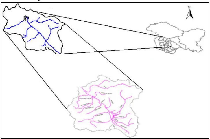
The present study was carried out in the upper Jhelum catchment. The study area spatially lies between 33° 21′ 54″ N to 34° 27′ 52″

N latitude and 74° 24′ 08″ E to 75° 35′ 36″ E longitude with a total area of 8600.78 sq.kms (Figure.1). It covers almost all the

is the largest urban centre in the valley is settled on both the sides of Jhelum River and is experiencing a fast spatial growth. Physical features of contrasting nature can be observed in the study area that ranges from fertile valley floor to snow-clad mountains and from glacial barren lands to lush green forests.

Figure 1.Location map of study area

III. DATA

The discharge data at Padshahibagh gauging station from 2001-2013 was procured from the Irrigation and Flood Control Department, Srinagar. The precipitation data at Srinagar, Pahalgam and Qazigund stations for years 2001-2013 was procured from Indian meteorological department (IMD) and national climate data centre (NCDC,US). Based on the availability of data the model was developed. Various rainfall events were selected from 2001-2013 and the models were developed for the same. The data sets for the years 2001-2009 were used for development/calibrating/training the models and these models were validated for various data sets achieved for 2010-2013.

IV. MULTIPLE LINEAR REGRESSION (MLR)

A Multiple Linear Regression Model is a linear Model that describes how a y-variable relates to two or more x-variables. The general structure of the model is as given below:

Y=βₒ+β₁X₁+β₂X₂+ …

Where, y is the dependent (or response) variable, x is independent (or predictor) variable .A linear model is one that is linear in the

beta coefficients, meaning that each beta coefficient simply multiplies to an x-variable.

The present study is under taken develop rainfall-runoff model in river Jhelum. Multiple Linear Regression and Artificial Neural Network Techniques will be used to develop the rainfall runoff models, to predict the runoff discharges at Padshahi Bagh station. A predictive analysis is used to determine the predictors which influence the runoff. After the model development the runoff at the Padshahi-Bagh station could then be predicted.

In this case, predicative analysis has to be applied for correctly modelling rainfall-runoff relationships. The follow equation shows relationships of rainfall and runoff

Q=f (Pt, P(t-1), P(t-2),….., P(t-m), Q(t-1), Q(t-2),…..,Q(t-n)

Where, Q(t) runoff at time t; Q(t-1): runoff at time t-1; Q(t-2): runoff at time t-2; Q(t-n): runoff at time t-n;) n: maximum steps of time lag of runoff. P(t): rainfall at time t; P(t-1): rainfall at time t-1; P(t-m): rainfall at time t-m. m: maximum steps of time lag of rainfall.

A. The Various Steps that were Undertaken to Develop the MLR model are given as under

1) The data was first normalized using MATLAB 7.10.0 software.

3) Using the Statistical tool box, regression was conducted on the data.

4) The regression analysis was done and regression equations were obtained for precipitation and runoff for the catchment.

5) The MLR model was validated by plotting the precipitation vs. runoff curve for the period 2010-2013 between predicted and

observed values.

6) The Analysis of Variance was done and R2 and Root Mean Squared Error (RMSE) were computed.

Figure 2. EXCEL worksheet showing regression between variables

V. RESULTS AND DISCUSSIONS

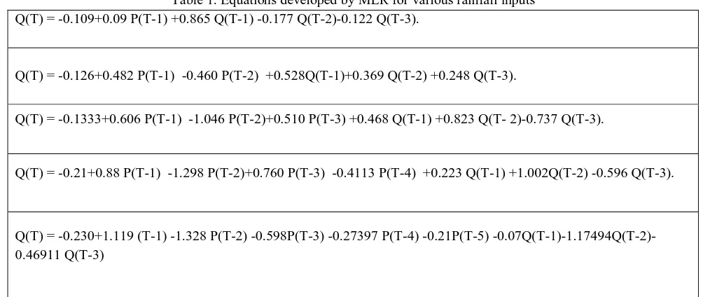
The number of input rainfall parameters were changed from P(t-1) to P(t-5) and multiple linear regressions were carried out. The MLR model was first trained for the years 2001-2010 and then validated for 2010-2013. The equations developed by MLR on changing the previous day rainfall inputs from one to five are given below in table 1.

Table 1. Equations developed by MLR for various rainfall inputs Q(T) = -0.109+0.09 P(T-1) +0.865 Q(T-1) -0.177 Q(T-2)-0.122 Q(T-3).

Q(T) = -0.126+0.482 P(T-1) -0.460 P(T-2) +0.528Q(T-1)+0.369 Q(T-2) +0.248 Q(T-3).

Q(T) = -0.1333+0.606 P(T-1) -1.046 P(T-2)+0.510 P(T-3) +0.468 Q(T-1) +0.823 Q(T- 2)-0.737 Q(T-3).

Q(T) = -0.21+0.88 P(T-1) -1.298 P(T-2)+0.760 P(T-3) -0.4113 P(T-4) +0.223 Q(T-1) +1.002Q(T-2) -0.596 Q(T-3).

After carrying out regression and validating the data the value of R2 and RMSE for different parameters were calculated as under:

Figure 3. Variation of R-square with different input vectors in MLR.

Figure 4. Variation of RMSE with different input vectors in MLR. 0.73

0.74 0.75 0.76 0.77 0.78 0.79 0.8 0.81 0.82 0.83 0.84

R-Square p(T-1)

p(T-1)… p(T-2)

p(T-1)…p(T-3)

p(T-1)… p(T-4)

p(T-1) …p(T-5)

0 0.5 1 1.5 2 2.5 3

MSE p(T-1)

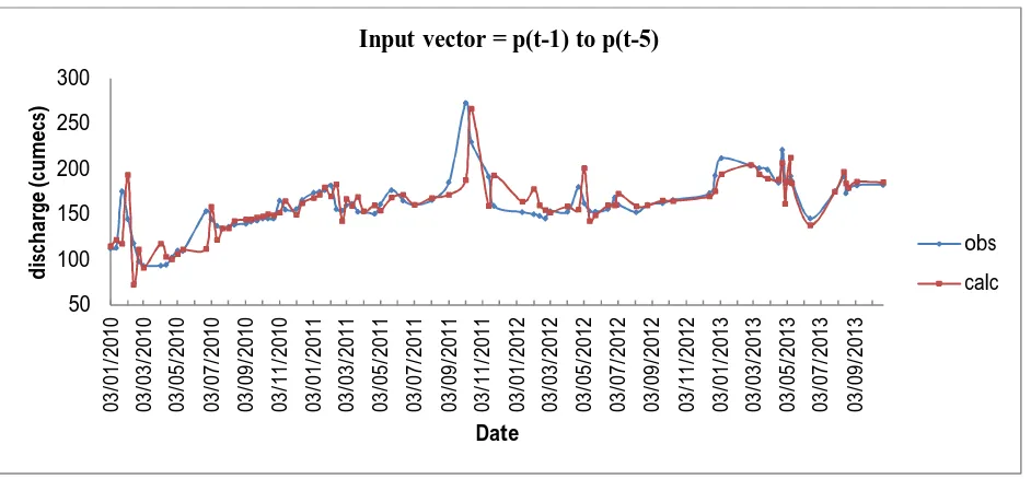
Figure 5. Observed vs. predicted discharge input P(t-1)…P(t-5).

VI. CONCLUSION

It was observed that the MLR model got simulated very well with a small value of MSE, RMSE a high value of R2, revealing that

the model is quite efficient in predicting the discharge of river Jhelum at Padshahi Bagh station based on the discharge of the upstream tributaries.

REFERENCES

[1] Abbott, M. B., Bathurst, J. C., Cunge, J. A., O’Connell, P. E., and Rasmussen, J.: An introduction to the European Hydrologic System Systeme Hydrologique Europeen, SHE, 1: History and philosophy of a physically based, distributed modelling system, J.Hydrol., 87, 45–59, 1986a.

[2] Abbott, M. B., Bathurst, J. C., Cunge, J. A., O’Connell, P. E., and Rasmussen, J.: An introduction to the European Hydrologic System Systeme Hydrologique Europeen, SHE, 2: Structure of a physically based, distributed modelling system, J. Hydrol., 87,61–77, 1986b.

[3] Bergstrom, S. and Forsman, A.: Development of a conceptual deterministic rainfall-runoff model, Nordic Hydrol., 4, 147–170, 1973.

[4] Bergstrom, S.: The HBV model, in: Computer models of watershed hydrology, edited by: Singh, V. P., Water Resources Publications,USA, 443–520, 199 [5] Beven, K. J.: Changing ideas in hydrology: the case of physically based models, J. Hydrol., 105, 157–172, 1989

[6] Beven, K. J.: Prophesy, reality and uncertainty in distributed hydrological modelling, Adv. Water Res., 16, 41–51, 1993.

[7] Beven, K. J., Calver, A., and Morris, E.: The Institute of Hydrology distributed model, Institute of Hydrology Report No. 98, UK,1987

[8] Beven, K. J., Lamb, R., Quinn, P., Romanowicz, R., and Freer, J.: TOPMODEL, in: Computer models of watershed hydrology, edited by: Singh, V. P., Water Resources Publications, USA,627–668, 1995

[9] Burnash, R. J. C., Ferral, R. L., and McGuire, R. A.: A Generalized streamflow simulation system – Conceptual modeling for digital computers, US Department of Commerce, National Weather Service and State of Califonia, Department of Water Resources,1973

[10] Burnash, R. J. C.: The NWS river forecast system – Catchment modelling, in: Computer models of watershed hydrology, edited by: Singh, V. P., Water Resources Publications, USA, 311–366, 1995.

[11] Calver, A and Wood, W. L.: The Institute of Hydrology distributed model, in: Computer models of watershed hydrology, edited by: Singh, V. P., Water Resources Publications, USA, 595–626,1995.

[12] Freeze, R. A. and Harlan, R. L.: Blueprint for a physically-based, digitally-simulated hydrologic response model, J. Hydrol., 9, 237–258, 1969.

[13] Grayson, R. B., Moore, I. D., and McMahon, T. A.: Physically based hydrologic modeling, 1, A terrain-based model for investigative purposes, Water Resour. Res., 28, 2639–2658, 1992a.

[14] Grayson, R. B., Moore, I. D., and McMahon, T. A.: Physically based hydrologic modeling, 2, Is the concept realistic?, Water Resour. Res., 28, 2659–2666, 1992b.

[15] Lindstrom, G., Johansson, B., Persson, M., Gardelin, M., and Bergstrom, S.: Development and test of the distributed HBV-96hydrological model, J. Hydrol., 201, 272–288, 1997

[16] Mehnaza Akhter.:Projection of future temperature and precipitation for Jhelum river basin in India using Multiple linear regression,Int.Journal of Engineering Research and Application,issue 6,(part-4)June 2017

[17] O’Connell, P. E. and Todini E.: Modelling of rainfall, flow and mass transport in hydrological systems: an overview, J. Hydrol., 175,3–16, 1996.

[18] Refsgaard, J. C. and Storm, B.: MIKE SHE, in: Computer models of watershed hydrology, edited by: Singh, V. P., Water Resources Publications, USA, 809– 846, 1995.

[19] Refsgaard, J. C., Storm, B., and Abbott, M. B.: Comment on “A discussion of distributed hydrological modelling” by K. Beven, in: Distributed hydrological modelling, edited by: Abbott, M. B.and Refsgaard, J. C., Kluwer Academic Publishers, Dordrecht,The Netherlands, 279–287, 199

[20] Todini, E.: The ARNO rainfall-runoff model, J. Hydrol., 175, 339–382, 1996. 50 100 150 200 250 300 03 /0 1/ 2 01 0 03 /0 3/ 2 01 0 03 /0 5/ 2 01 0 03 /0 7/ 2 01 0 03 /0 9/ 2 01 0 03 /1 1/ 2 01 0 03 /0 1/ 2 01 1 03 /0 3/ 2 01 1 03 /0 5/ 2 01 1 03 /0 7/ 2 01 1 03 /0 9/ 2 01 1 03 /1 1/ 2 01 1 03 /0 1/ 2 01 2 03 /0 3/ 2 01 2 03 /0 5/ 2 01 2 03 /0 7/ 2 01 2 03 /0 9/ 2 01 2 03 /1 1/ 2 01 2 03 /0 1/ 2 01 3 03 /0 3/ 2 01 3 03 /0 5/ 2 01 3 03 /0 7/ 2 01 3 03 /0 9/ 2 01 3 d is ch ar ge (c u m e cs ) Date

Input vector = p(t-1) to p(t-5)

obs