Simulation of Hydraulic Parameters of Desapatrunipalem (GVMC, Visakhapatnam) Water Distribution Network by using EPANET

Simulation of Hydraulic Parameters of

Desapatrunipalem (GVMC, Visakhapatnam)

Water Distribution Network by using EPANET

Y. Roopavathi1, Ch. Ramesh Naidu2

1

Post graduate student, 2Professor, Department of Civil Engineering, Gayatri Vidya Parishad College of Engineering (A), Visakhapatnam-530048, India

Abstract: The present existing water supply system adopted in Desapatrunipalem is an irregular supply and the network implemented is a dead end/Tree system. In order to fulfil the water demand of the continuously growing population, it is essential to provide the sufficient and uniform quantity of water through thedesigned network. For this purpose the details provided by the GVMC(Projects Department), Visakhapatnam have been followed. The general features of the area likemain water source, population of the area, demand of water, distribution network and water tanks are essential for effiecient design ofsystem. According to the GVMC the per capita consumption of water is 100 lpcd and design has been made accordingly. This work highlights the process carried for design of water supply system for Desapatrunipalem with the help of software “EPANET”.Thisdesign of the water supply scheme for proper supply of water is efficient to meet the daily requirement of water in this area. The design is done based on population growth rate, and the developments inthe village. This analysis provides the information about various demands, losses, pressures and head ofthe network.

Keywords: Water supply, Population Forecast, Water Demand, Network Analysis and EPANET Simulation

I. INTRODUCTION

Water distribution system, a hydraulic infrastructure consisting of elements such as pipes, tanks, reservoirs, pumps and valves etc., is crucial to provide water to the consumers. Effective water supply system is of paramount importance in designing a new water distribution network or in expanding the existing one. Distribution networks are an essential part of all water supply systems. Distribution system costs within any water supply scheme may be equal to or greater than 60 % of the entire cost of the project. A water distribution system is a collection of hydraulic control elements jointly connected to convey quantities of water from sources to consumers. Simulation of water distribution systems using computer technique has reached a mature stage of development. Due to the advent of Geographical Information Systems (GIS), it is possible to visualize, and model the entire cycle of water supply network from source to household. The network system must be modeled, analyzed, and its performance is evaluated under the various physical and hydraulic parameters or conditions. This process is called as “Simulation’. EPANET is a computer program that performs extended period simulation of hydraulic and water quality behavior within pressurized pipe networks. EPANET tracks the flow of water in each pipe, the pressure at each node, the height of water in each tank, and the concentration of a chemical species throughout the network during a simulation period comprised of multiple time steps.

A. Objectives

Objectives of the study are as follows.

1) Generation of thematic layers for Desapatrunipalem village by Digitization process using GIS.

2) Population Forecasting by different methods.

3) Design of pipe network considering nodal demand for the future demand.

4) Simulation of the water distribution network for various hydraulic parameters.

5) Verifying the output values with standard values of pressure, velocity and unit headloss.

II. STUDY AREA

Desapatrunipalem is a village in Gajuwaka Mandal part of 55th Ward and Zone 5 of Visakhapatnam district, Andhra Pradesh state,

pipe network has to be simulated. The present system is not at all sufficient to meet the demand of the people. This village was merged in GVMC in the year 2004 and water supply for this village is an intermittent supply running by 3 bore wells by Pumping system. To carry out this study existing water distribution network map which was prepared in 2008 is collected from the projects department of GVMCwhich contains the basic data like major nodes, land marks, road network, ELSRs, pipes, valves, pipe diameters, pumps etc., This study is carried out as part of ongoing project of JNNURM by Greater Visakhapatnam Municipal Corporation (GVMC), Visakhapatnam, India in a view of providing sufficient water supply to the village from Yeleru canal. The total population of the village is 5832 as per the Census 2011. The village consists of 1531 households.

III. METHODOLOGY A. Population Forecasting

The existing population data for last 2 decades is as follows, for 1991, 2001 and 2011 population values are 2029, 3186 and 5832 souls and no. of households are 465, 1003 and 1531 respectively. For this project, both Geometrical and Incremental increase methods were used because the population growth trend follows these methods.

Table 1: Forecasted Population Data

Year Geometrical Increase Method Incremental Increase Method

2021 9843 9222

2031 16613 12737

2041 28039 16200

2051 47323 19612

B. Water Demand calculation

Domestic water demand for GVMC is 100lpcd and an additional amount of 15% will be supplied as unaccounted flow.

For designedpopulation i.e., 9222, calculated water demand is 1.06 MLD also represented as 12.27 lt/sec which can be calculated according to the formula i.e.,

Water demand Q = Population x Per capita demand

Table 2: Nodal demand for 3 decades Nodal Demand (LPS)

S No Representative

Length (m)

2021 2031 2041 2051

1 0 0.00 0.00 0.00 0.00

2 70 0.05 0.06 0.08 0.10

3 217 0.15 0.20 0.24 0.30

4 292 0.20 0.26 0.32 0.41

5 161 0.11 0.14 0.18 0.23

6 220 0.15 0.20 0.24 0.31

7 235 0.16 0.21 0.26 0.33

8 73 0.05 0.07 0.08 0.10

9 103 0.07 0.09 0.11 0.14

10 61 0.04 0.05 0.07 0.09

11 51 0.04 0.05 0.06 0.07

12 52 0.04 0.05 0.06 0.07

13 54 0.04 0.05 0.06 0.08

14 50 0.04 0.05 0.06 0.07

15 48 0.03 0.04 0.05 0.07

17 54 0.04 0.05 0.06 0.08

18 79 0.06 0.07 0.09 0.11

19 61 0.04 0.05 0.07 0.09

20 42 0.03 0.04 0.05 0.06

21 43 0.03 0.04 0.05 0.06

22 42 0.03 0.04 0.05 0.06

23 53 0.04 0.05 0.06 0.07

24 33 0.02 0.03 0.04 0.05

25 46 0.03 0.04 0.05 0.06

26 48 0.03 0.04 0.05 0.07

27 45 0.03 0.04 0.05 0.06

28 49 0.03 0.04 0.05 0.07

29 55 0.04 0.05 0.06 0.08

30 43 0.03 0.04 0.05 0.06

31 46 0.03 0.04 0.05 0.06

32 23 0.02 0.02 0.03 0.03

33 25 0.02 0.02 0.03 0.04

C. Network generation, modelling and simulation

The digitized Google map shape (*.shp) file is converted to bitmap image (.bmp) file. Finally this .bmp file is used as a backdrop in EPANET software. This allows us to assign prefixes to the junctions and pipes and to obtain a working model of the system in EPANET. Now the pipe network layout and distribution is drawn along road network. The junctions are created with their respective base demand. These junctions are joined together with pipes of varying length and diameter. The length of the pipe lines between the nodes are arrived from Google earth and used in EPANET. The valves are also used in the network system to regulate the flow. After a working model of the network is generated in EPANET, the next step is to assign water demand and elevation to the different nodes along with pipe characteristics such as pipe length, pipe diameter and roughness coefficients to the respective pipes. The process of modelling a network using EPANET involves input of the parameters or variables that most closely describe the operation of the actual system.

Fig2. 2051 report of water distribution network

IV. RESULTS/ FINDINGS

The output results computed for junctions are hydraulic head, pressure and age. The junction report for simulation of peak hour water demand, i.e.5:30–8:30AM is shown.The highest pressure achieved during simulation process is 25.99m. 35.4% of the total nodes have negative pressure, 20.1% of the total nodes have pressure less than 10m, 33.1% of the total nodes have pressure greater than 10m and 11.4% of the total nodes has pressure greater than 20m.

The output results computed for the pipes are flow rates, friction factor, velocity and unit headloss. The pipe report for simulation of peak hour water demand, i.e.5:30–8:30AM is shown. The distribution of velocity during the peak water demand hour shows that177 links have a velocity less than 0.5m/s, 73 links have a velocity less than 2m/s, while 25 links have velocity greater than 2m/s. The pressures and velocities which are obtained by simulation are not sufficient to run the network. Hence, the network has revised as per the standards of IS 4895:2000 and CPHEEO.

A. 2051 Revised Network By Epanet

During the network simulation, changes in selected parameters such as head, flow, velocity, unit headloss and water pressure at various nodes and links were observed. The water distribution network of Desapatrunipalem consists of 275 pipes of uniform material, 263 junctions, 8 valves and 1 elevated service reservoir from which water is distributed to the entire network. The pipes used in the network system are of different diameter ranges from 90mm to 315mm (as per IS 4895:2000). The PVC pipes having roughness coefficient of 145 are used throughout the network system (as per standards of CPHEEO).

B. Revised Network Output

The revised network output values of pressure, velocity, flow, head and unit headloss are following the standard values and the pressure values of nodes are ranges from 10.32 to 29.87, 20% of nodes are having pressure > 10m and 80% of nodes having pressure > 20m and all the pipes are having velocity values between 0.5m/s to 2m/s and unit headloss values <5m/km which are given below in tabular form.

1) Nodes Report: The output results computed for nodes are hydraulic head, pressure and age. The junction report for simulation of peak hour water demand, i.e.5:30–8:30AM is shown.The highest pressure achieved during simulation process is 29.87m. 21.7% of the total nodes have pressure greater than 10m and 78.3% of the total nodes has pressure greater than 20m.

Node ID

Demand

(LPS) Head (m) Pressure(m) Age

Junc 21 0.6 58.88 10.32 0

Junc 50 0.4 58.88 10.38 0

Junc 51 0.2 58.87 10.52 0

Junc 22 0.6 58.87 10.55 0

Junc 20 0.6 58.92 11.05 0

Junc 49 0.4 58.92 11.43 0

Junc 47 0.9 59.03 12.09 0

Junc 18 1.1 59.07 12.10 0

Junc 36 0.4 59.23 12.98 0

Junc 17 0.8 59.23 13.15 0

Junc 35 0.4 59.36 13.73 0

Junc 16 0.6 59.36 13.83 0

Junc 37 0.5 59.49 14.09 0

Junc 15 0.7 59.5 14.77 0

Junc 28 0.7 59.61 15.75 0

Junc 27 0.6 59.63 15.77 0

Junc 38 0.1 59.61 15.75 0

Junc 48 0.8 58.96 11.47 0

Junc 54 0.6 60.28 17.92 0

Junc 15 0.7 59.5 14.77 0

Junc 14 0.7 59.62 15.42 0

Junc 65 0.6 59.92 21.7 0

Junc 70 0.7 59.81 21.83 0

Junc 27 0.6 59.63 15.77 0

Junc 13 0.8 59.75 15.85 0

Junc 19 0.9 58.99 16.07 0

Junc 24 0.5 59.75 16.65 0

Junc 12 0.7 59.88 16.72 0

Junc170 0.2 58.56 29.76 0

Junc164 1.1 57.82 29.84 0

Junc149 0.2 58.67 29.87 0

Junc 76 0.8 58.55 29.81 0

Junc269 1.7 61.47 21.22 0

2) Links Report: The output results computed for the pipes are flow rates, friction factor, velocity and unit headloss. The pipe report for simulation of peak hour water demand, i.e.5:30–8:30AM is shown. The distribution of velocity during the peak water demand hour shows that 177 links have a velocity less than 0.5m/s, 73 links have a velocity less than 2m/s, while 25 links have velocity greater than 2m/s.

Link ID Flow

(LPS) Velocity (m/s) Unit Headloss (m/km) Friction Factor

Pipe255 0.1 0.01 0.00 0.000

Pipe236 0.31 0.01 0.00 0.000

Pipe194 0.2 0.01 0.00 0.000

Pipe 143 0.6 0.09 0.14 0.028

Pipe 149 1.1 0.12 0.16 0.026

Pipe 85 0.68 0.11 0.18 0.028

Pipe 75 1.51 0.24 0.78 0.025

Pipe 138 1.6 0.25 0.87 0.024

Pipe 159 2.0 0.31 1.32 0.024

Pipe 31 2.47 0.39 1.95 0.023

Pipe 53 4.41 0.46 2.14 0.022

Pipe 55 6.5 0.53 2.36 0.021

Pipe 35 0.5 0.08 0.10 0.029

Pipe 39 0.5 0.08 0.10 0.029

Link ID Flow (LPS) Velocity (m/s) Unit Headloss (m/km) Friction Factor

Pipe 58 8.65 0.7 4.01 0.02

Pipe 11 16.6 0.83 4.03 0.019

Pipe 244 6.21 0.65 4.04 0.02

Pipe 64 6.21 0.65 4.05 0.02

Pipe 196 24.7 0.97 4.74 0.018

Pipe 206 4.00 0.63 4.77 0.021

Pipe 93 58.9 1.2 4.79 0.016

Pipe 10 4.07 0.64 4.93 0.021

Pipe 219 9.70 0.79 4.96 0.019

Pipe 171 4.10 0.64 4.99 0.021

Pipe 98 213.9 1.7 5.29 0.014

Pipe 1 214.9 1.71 5.33 0.014

Pipe 67 1.46 0.23 0.73 0.025

Pipe 72 1.48 0.23 0.76 0.025

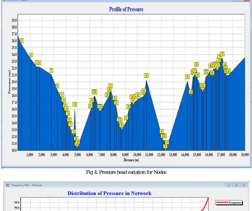
C. Nodal pressure result for current demand:

Fig 4. Pressure head variation for Nodes

Fig 6. Velocity variation for pipes

D. Velocity results for current demand

The velocities range from 0.01 m/s to 1.71m/s are shown in Fig 6. The minimum and maximum velocity in the network should be 0.5 m/s and 2.0m/s, respectively. The velocity of flow in the network is sufficient except in some pipes due to the dead ends. Looping the network is useful to overcome this drop in velocity near the dead ends.

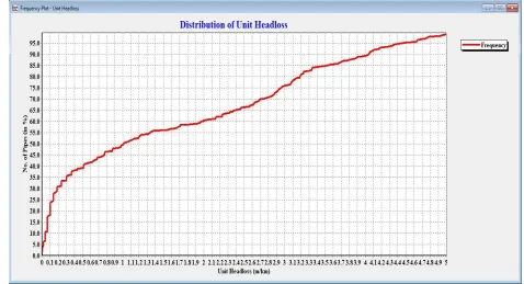
E. Unit Headloss results for current demand

The unit headloss results are shown in the Fig 7, all the pipes are having the unit headloss values in acceptable limit i.e., less than 5m/km.

V. CONCLUSIONS The following conclusions can be drawn from the study

A. The residual pressure at all nodes is found to be greater than 10.00 m. Hence, the flow can takes place easily.

B. The main focus of this study is to analyze the water distribution network and identify deficiencies (if any) in its analysis, implementation, usage and to make sure that the resulting pressures at all the junctions are should be in the range of 10m to 30m and the flows with their velocities at all pipes are < 2 m/s and Unit Headloss in all pipes is < 5m/km.

C. It was found that the resulting pressures at all the junctions are found to be greater than 10 m and less than 30m and the flows with their velocities at all pipes are in the range of 0.1–2 m/s and Unit Headloss in all pipes is < 5m/km, which is adequate enough to provide water to the entire study area.

D. The assumed diameters of all pipes (90mm to 315mm) are sufficient to withstand for the pressure of the entire network.

E. The pressure values of nodes are ranges from 10.32 to 29.87, 20% of nodes are having pressure > 10m and 80% of nodes having pressure > 20m and all the pipes are having velocity values between 0.5m/s to 2m/s and unit headloss values <5m/km. F. This study has been carried out by developing various thematic maps and integrating various field and administrative

information in GIS environment. With the help of the GIS studies and EPANET modification of the water distribution network has been suggested for better management of the area.

G. Overall this study will be helpful for the Municipality to aware of the new demands and plan the network according to it.

VI. ACKNOWLEDGEMENT

The authors are very grateful to Gayatri Vidya Parishad College of Engineering (Autonomous) which provided us this wonderful opportunity to carry out the current work and for providing encouragement to write this paper. The authors are thankful to projects department ofGreater Visakha Municipal corporation (GVMC) for the encouragement and technical support extended in the form of by providing vital information useful for this paper.

REFERENCES

[1] R. Sathyanathan, Mozammil Hasan, V.T. Deeptha (2016), Water Distribution Network Design for SRM University using EPANET, Asian Journal of Applied Sciences (ISSN: 2321 – 089),Volume 04 – Issue 03, June 2016

[2] G. Anisha, A. Kumar, J. Ashok Kumar, P. Suvarna Raju (2016), Analysis and Design of Water Distribution Network Using EPANET for Chirala Municipality in Prakasam District of Andhra Pradesh, International Journal of Engineering and Applied Sciences (IJEAS) ISSN: 2394-3661, Volume-3, Issue-4, April 2016 [3] Dr. H. Ramesh, L. Santhosh and C. J. Jagadeesh (2012), Simulation of Hydraulic Parameters in Water Distribution Network Using EPANET and GIS,

International Conference on Ecological, Environmental and Biological Sciences (ICEEBS'2012) Jan. 7-8, 2012 Dubai

[4] D. Ram Mohan Rao, Zameer Ahmed, Dr. Y. Ellamraj, Dr. D. Ram Mohan Reddy (2015), EPAnet Demand Calculation Methods and Implications, International Journal of Scientific Engineering and Research (IJSER), ISSN (Online): 2347-3878, Volume 4 Issue 11, November 2016

[5] Piplewar S.K, Chavhan Y.A (2013), Design of Distribution Network for Water Supply Scheme at Pindkepar Village by Branch Software, Journal of Engineering Research and Applications, ISSN : 2248-9622, Vol. 3, Issue 5, Sep-Oct 2013, pp.854-858

[6] KakadiyaShital, MavaniKrunali, Darshan Mehta, Vipin Yadav (2016), Simulation of Existing Water Distribution Network by using EPANET: A Case Study of Surat City, Global Research and Development Journal of Engineering | Recent Advances in Civil Engineering for Global Sustainability | e-ISSN: 2455-5703, March 2016

[7] Shivalingaswami.S.Halagalimath, Vijaykumar.H, Nagaraj.S.Patil (2016), Hydraulic modeling of water supply network using EPANET, International Research Journal of Engineering and Technology (IRJET) e-ISSN: 2395 -0056, p-ISSN: 2395-0072, Volume: 03 Issue: 03 | Mar-2016

[8] Maulik Joshi, ShilpaChavda, DharmeshRajyaguru, Sohamsarvaiya (2014), Design of Water Distribution Supply Network For Kuchhadi Village, Paripex - Indian journal of research, ISSN - 2250-1991, Volume : 3 | Issue : 2 | Feb 2014

[9] IS 4895:2000, Unplasticized PVC pipes for potable water supplies -- specification, (Third Revision), March 2005

[10] The Central Public Health and Environmental Engineering Organization (CPHEEO), Manual on water supply & Treatment, Third Edition (Revised & Updated), Ministry of Urban development, New Delhi, May 1999.

[11] ERDAS Field Guide, http://web.pdx.edu/~emch/ip1/FieldGuide.pdf