The compact genetic algorithm for likelihood estimator of first order moving average model

The Compact Genetic Algorithm for Likelihood

Estimator of First Order Moving Average Model

Rawaa Dawoud Al-Dabbagh

, Dr. Mohd. Sapiyan Baba

, Dr. Saad Mekhilef

, Azeddien Kinsheel

Department of Artificial Intelligence 2

Department of Electrical Engineering 3

Department of Engineering Design and Manufacturing University of Malaya

Kuala Lumpur, Malaysia

[email protected], [email protected], [email protected], [email protected]

Abstract—Recently Genetic Algorithms (GAs) have

frequently been used for optimizing the solution of estimation problems. One of the main advantages of using these techniques is that they require no knowledge or gradient information about the response surface. The poor behavior of genetic algorithms in some problems, sometimes attributed to design operators, has led to the development of other types of algorithms. One such class of these algorithms is compact Genetic Algorithm (cGA), it dramatically reduces the number of bits reqyuired to store the poulation and has a faster convergence speed. In this paper compact Genetic Algorithm is used to optimize the maximum likelihood estimator of the first order moving avergae model MA(1). Simulation results based on MSE were compared with those obtained from the moments method and showed that the Canonical GA and compact GA can give good estimator of ࣂ෡ for the

MA(1) model. Another comparison has been conducted

to show that the cGA method has less number of function evaluations, minimum searched space percentage, faster convergence speed and has a higher optimal precision than that of the Canonical GA.

Keywords-Moving Average (MA), Likelihood Function,

Moment Estimation Method, Canonical Genetic Algorithm (CGA), compact Genetic Algorithm (cGA), Mean Square Error (MSE).

I. INTRODUCTION

One of the most famous procedures for the solution of optimization problems is Genetic Algorithms (GAs). GA is composed mainly of three steps: recombination, crossover and mutation. By maintaining a population of solutions, GA can be viewed as implicitly modeling of the solutions seen in the search process. In the standard GA, new solutions are generated by applying randomized recombination operators on two or more high-quality individuals of the current population [1]. These recombination operators, such as one-point, two-point or uniform crossover, randomly selected non- overlapping subsets of two “parent” solutions to form “children” solutions.

The poor behavior of genetic algorithms in some problems, sometimes attributed to designed operators, has led to the development of other types of algorithms such as the Probabilistic Model Building Genetic Algorithms (PMBGAs) or Estimation of Distribution Algorithms (EDAs). They are a class of algorithms which have been developed recently to preserve the building blocks [2]. The principal concept in these new techniques is to prevent the distribution of partial solutions contained in a solution by building a probabilistic model [2] [3] [4]. To name just a few, instances of EDA algorithms include the Population-based Incremental Learning (PBIL) [5] [6] and the compact Genetic Algorithm (cGA) [7]. The compact GA represents the population as a probability (distribution) vector (PV) over the set of solutions and is operationally equivalent to the order-one behavior of the simple GA with uniform crossover. It processes each gene independently and requires less memory than simple GA [7] [2]. As a case study to investigate the relative performance of cGA for optimizing the solution of estimation problem, we have utilized cGA for optimizing the maximum likelihood ݈݊൫ܮሺߠǡ ߪ_௔ଶሻ൯ function of the first order moving average model MA(1).

A time series is an ordered sequence of observations in an equal interval space; this ordering is generated through time or other dimensions such as sapce. Time series occur in a variety of fields (such as engineering, economics and agriculture). As one of the distinguished stochastic models which represent time series is the simple moving average and it is also called a first order moving average, denoted by MA(1) because it contains just one parameter, ߠ. A generalization of the MA(1) model is the ݍ௧௛ order moving average which is denoted by MA(q) and takes the formula [8]

ݖ_௧ൌ ܽ_௧െߠ_ଵܽ_௧ିଵെ ڮ െߠ_௤ܽ_௧ି௤ (1)

ݖ_௧ൌ ߠሺܤሻܽ_௧ (2)

ߠሺܤሻ ൌ ͳ െߠଵܤ െ ڮ െߠ௤ܤ௤ିଵ

process is stationary for any value of ߠ_ଵǡ ߠ_ଶǡ ǥ ǡ ߠ_௤, that is, the mean and the variance of the underlying process are constant and auto-covariance’s depends only on the time lag. But many economic and business time series are somtimes considered to be non-stationary. Non-stationary time series can occur in many different ways. Sometimes the series has a non-stationary behavior about a fix mean, and hence its behavior can be represented by a model which calls for ݀௧௛ difference of the process to be stationary. In practice d is usually 0, 1, or at most 2. The difference provides a powerful model for describing stationary and non-stationary time series and it is called an integrated moving average (IMA) process or ARIMA of order ሺͲǡ ݀ǡ ݍሻ. The process which is defined by first order, is known as ARMAሺͲǡ ݀ǡ ݍሻ, it takes the formula

ݓ_௧ൌ ܽ_௧െߠ_ଵܽ_௧ିଵ (3)

or in its operator form:

ݓ_௧ൌ ߠሺܤሻܽ_௧ (4)

where ݓ_௧ൌ ׏ௗݖ_௧ and the moving average operator ߠሺܤሻ ൌ

ͳ ൅ ߠ_ଵܤ ൅ ߠ_ଶܤଶ_{൅ ڮ ൅ ߠ}

௤ܤ௤, here the moving average process is stationary for any values of ߠ_ଵǡ ߠ_ଶǡ ǥ ǡ ߠ_௤.

This model will be invertible if the root of ሺͳ െ ߠ_ଵܤ ൌ Ͳሻ lies outside the unit circle; an inertible MA is time reversible, so we can get that ȁߠ_ଵȁ ൏ ͳ. Moments of this stationary model are:

Mean Function

E(Z) = 0 (5) Variance Function

ߛ_଴ൌ ݒܽݎሺݖ_௧ሻ ൌ ሺͳ ൅ߠ_ଵଶሻߪ_௔ଶ (6)

Auto-Covariance Function

ߛ_௞ ൌ ൤െߠଵߪ௔ଶ ݇ ൌ ͳ

Ͳ ݇ ൐ ͳ൨ (7)

Auto-Correlation Function

ߩ_௞ൌ ቎

ͳ ݇ ൌ Ͳ

ିఏభ

ଵାఏభమ ݇ ൌ ͳ

Ͳ ݁Ǥ ݓ

቏ (8)

We can show that the marginal distribution of time series that has MA(1) model is ݖ_௧̱ܰሺͲǡ ሺͳ ൅ ߠ_ଵଶሻߪ_௔ଶሻ if

ܽ௧̱ܰሺͲǡ ߪ௔ଶሻ. Estimation is the second step in analysis of the time series. It indicates an effecient use of the data to make inferences about the parameters conditional to the adequacy of the entrtained model. ARMA models can be difficult to estimate if the parameter estimates are not within the appropriate range, a moving average model’s residual terms will grow exponentially. The calculated residuals for later observations can be very large or can overflow. This can happen either because of improper starting values being used or because the iterations moved away from reasonable values. Moreover, our model is nonlinear because ܽ_௧ൌ

_ଵିఏଵ

భ஻, so there is no direct method that can handle these

limitations, but all suitable methods are indirect methods

(Iterative method) which start with an initial value and then this value is modified iteratively by using some numerical algorithms. The numerical method gives an approximate estimator with some accuracy.

Recently, B. Hussain [9] [10] proposed the use of Canonical Genetic Algorithm (CGA) for optimizing the maximum likelihood function ݈݊൫ܮሺߠǡ ߪ_௔ଶሻ൯ of the first order moving average MA(1) model. And its results were compared with the results obtained by the moment estimator method.

In this paper we introduce a new evolutionary way to estimate the same model by using the compact Genetic Algorithm (cGA). Droste [11] proofed that cGA is applicable to be used for optimizing most of the linear functions such One-Max in the optimal expected runtime. In this paper we are interested in the behavior of the cGA for non-linear functions in comparison with CGA according to the number of function evaluations taken, solution quality, the percentage of the search space searched until convergence and the convergence speed.

The rest of the paper is organized as follows. Section 2 explains the problem formulation of maximum likelihood estimator. Section 3 briefly describes the standard cGA. Section 4 presents the simulation results obtained from applying CGA, cGA and moment method for optimizing the model under study. Section 6 concludes the paper.

II. PROBLEM FORMULATION

Maximum likelihood estimator (MLE) is a standard approach to parameter estimation and inference in statistics; it is a method that finds the most likely value for the parameter based on the data set collected, in particular in non-linear modeling with non-normal data. MLE has many optimal properties in estimation: sufficiency (complete information about the parameter of interest contained in its MLE estimator); consistency (true parameter value that generated the data recovered asymptotically, i.e. for data of sufficiently large samples); efficiency (lowest-possible variance of parameter estimates achieved asymptotically); and parameterization invariance (same MLE solution obtained independent of the parameterization used) [12].

Assume that a time series which is denoted by

ݖ_ିௗାଵǡ ǥ ǡ ݖ_଴ǡ ݖ_ଵǡ ݖ_ଶǡ ǥ ǡ ݖ_௡ is generated by an IMA(1,1) model over N= n + d original observations z. From these observations, a series ݓ ൌ ሼݓ_ଵǡ ݓ_ଶǡ ǥ ǡ ݓ_௡ሽ of n = N – d is generated where ݓ_௧ൌ ߘௗݖ_௧and n is the sample size. The stationary mixed ARMA(0,1) model in Eq.7 is rewritten as [13]

ܽ_௧ൌ ݓ_௧൅ߠ_ଵܽ_௧ିଵ (9)

where ܧሺݓ_௧ሻ ൌ Ͳ. Suppose that ሼܽ_௧ሽhas the normal ditribution with zero mean and constant variance equal to ߪ_௔ଶ

, then the likelihood function can be written as follows [13]:

ܮ ൌ ሺʹߨߪଶሻି೙మหܯሺ଴ǡଵሻห భ

మ_{݁ݔ݌ ቀ}ିௌሺఏభሻ

ଶఙೌమ ቁ (10)

The logarithmic likelihood function is given by:

ܮ݊ሺܮሻ ൌ െ௡

ଶሺʹߨߪ௔ሻ ൅ ଵ

ଶ݈݊ሺͳ െ ߠଵଶሻ െ ௦ሺఏభሻ

where

ܵሺߠ_ଵሻ ൌ σ௡_௧ୀଵܽ_௧ଶሺߠ_ଵȁݖ_଴ǡ ߠ_ଵǡ ݖሻ (12)

is the sum squares errors and ሾܽ_௧ȁߠ_ଵǡ ݓሿ ൌ ܧሾܽ_௧ȁߠ_ଵǡ ݓሿ denotes the expectation of ܽ_௧ conditional on ߠ_ଵand w. The sum squares of errors can be found by unconditional calculation of the [a]’s which are computed recursively by taking expectations in Eq.12, it is also called Least Square Estimate (LSE) in which the parameter estimated is obtained my minimizing the sum of square in Eq.12, it usually provides very close approximation to the maximum likelihood estimator. Back-forecasting is a popular technique, it estimates the parameters which are crudely put into the model and run backwards in time; a back-calculation provides the values ൣݓ_ି௝൧ǡ ݆ ൌ Ͳǡͳǡʹǡ ǥthis back-forecasting is needed to start off the forward recursion. For moderate and large values of n, Eq.12 is dominated by ܵሺߠ_ଵሻȀʹߪ_௔ଶ and thus the contours of the unconditional sum squares function in the space of the parameters ߠ are very nearly contours of likelihood and log-likelihood.

For a causal and finite auto-regressive equation, the method of moment estimators according to the Yule-Walker equations almost coincides with the least squares or maximum Gaussian likelihood estimators and their consistency as well as their asymptotic normality may be established. The standard Yule-Walker equations, as they are known for an auto-regression, are generalized to involve the moments of a moving-average process indexed on any number of dimensions [14]. It is obtained by equating a sample moment such as sample meanݖഥ, sample varianceߛෝ_଴, and sample ACF (Auto-correlation Function) ߩො_௜ to their theoretical values counterparts and solving the resultant equations.

For the presented model, the estimate of parameters can be obtained by equating sample moments to their theoretical values. Approximate values for the parameters are obtained by substituting the estimators ݎ_௞ forߩ_௞.

ߩො_௞ൌ ݎ_௞ൌ σ೙షೖ೟సభ_σሺ௭೟ି௭ҧሻሺ௭_ሺ௭ ೟శೖି௭ҧሻ

೟ି௭ҧሻ ೙

೟సభ (13)

Hence, from Eq.8 and the correlation function ߩ ൌ ିఏ ଵାఏభwe

get [13]:

ߩො_ଵൌ ݎ_ଵൌ ିఏ෡భ

ଵାఏ෡_భమ (14)

and ߠ෠_ଵൌ ିଵേටଵିସ௥భ

మ

ଶ௥భ (15)

where ߠ෠_ଵ is the value that makes ඥͳ െ Ͷݎ_ଵଶ> 0 and หߠ෠ห ൏ ͳ.

III. THE COMPACT GENETIC ALGORITHM (cGA) The compact Genetic Algorithm (cGA) is similar to the PBIL (population Based Incremental Learning) but requires fewer steps, fewer parameters and less of a gene sample [11].

The cGA manages its population as a probability vector (PV) over the set of solutions (i.e., only models its existence), therby mimicking the order-one behavior of the sGA with uniform crossover using a small amount of memory [1] [15].

Figure 1. Pseudo code fashion of the cGA

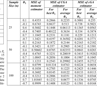
Figure 1 and 2 describes the pseudo-code and flowchart of the cGA. The values of PV ݌_௜א ሾͲǡͳሿ, ׊_௜ൌ ͳǡ ǥ ǡ ݈, where l is the number of genes (i.e., the length of the chromosome), measures the proportion of “1” alleles in the ݅௧௛ locus of the simulated population [2][15].The PV is initially assigned 0.5 to represent a randomly generated population. In every generation (i.e., iteration), competing chromosomes are generated on the basis of the current PV, and their probabilities are updated to favor a better chromosome (i.e, winner). It is noted that the generation of chromosomes from PV simulates the effects of crossover that leads to a decorrelation of the population’s genes. In a simulated population of size n, the probability ݌_௜ is increased (decreased) by ͳ ݊ൗ when the ݅௧௛ locus of the winner has an allel of “0”(“1”). If both the winner and the loser have the same allele in each locus, then the probability remains the same. This scheme is equivalent to (steady-state) pair-wise tournament selection [1]. The cGA is terminated when all the probabilities converge to zero or one. The convergent PV itself represents the final solution. It seen that the cGA requires ݈ ൈ݈݋݃_ଶሺ݊ ൅ ͳሻ bits of memory while the sGA requires ݈ ൈ ݊ bits [1]. Thus, large population size can be effectively exploited without unduly compromising on memory requirements [15].

A. Individual Initialization and Encoding:

Certain restrictions are defined on the encoding scheme:

1. cGA needs in every step two random numbers, each having a bit-string (0’s and 1’s) of fixed length l=15 bits. Two individuals a and b are generated: they are two identical chromosomes working in parallel, but using different initial seeds. Each individual affectionately known as a critter represents an element with the domain of the

Parameters. n: population size l: chromosome length

Step1. Initialize probability vector For i: = 1 to l do p[i]:= 0.5;

Step2. Generate two chromosomes from the probability vector a:= generate(p); b:= generate(p)

Step3. Let them compete

winner, loser := compete (a, b);

Step4. Update the probability vector fori:=1 to l do

if winner [i]

≠

if winner[i] == 1 then p[i]:= p[i] + 1/n

else p[i] := p[i] – 1/n ;

Step5. Check if the probability vector has converged. Go to Step 2, if it is not satisfied.

Yes

Yes

Yes No

No

No

solution space of the optimization problem. The chromosome of a given critter is the only source for of all the information about the corresponding solution. To apply the cGA to real-values parameters optimization problems of the form

݂ ׷ ςሾݑ௜ǡ ݒ௜ሿ ՜ ܴሺݑ௜൏ ݒ௜ሻ, the bit-strings is logically divided into n segments of (in most cases) equal length ݈_௫ሺ݈ ൌ ݈݊_௫ሻ and each segment is interpreted as the binary code of the corresponding object variable ݔ_௜א ሾݑ_௜ǡ ݒ_௜ሿ. A segment decoding function ߁௜ǣ ሼͲǡͳሽ௟ೣ_{՜ ሾݑ௜ǡ ݒ௜}ሿ_{typically looks like}

߁௜൫ܽ_௜ଵܽ_௜ଶǥܽ_௜௟ೣ൯ ൌ ݑ_௜൅௩೔ି௨೔

ଶ೗_௫ିଵൣσ ܽ௜௝ʹ௝ିଵ൧ ,

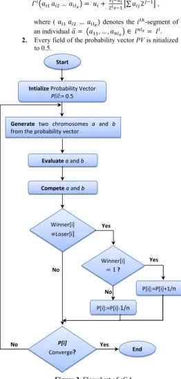
where ( ܽ_௜ଵܽ_௜ଶǥܽ_௜௟ೣሻ denotes the ݅௧௛-segment of an individual ܽറ ൌ ൫ܽ_ଵଵǡ ǥ ǡ ܽ_௡௟ೣ൯ א ݈௡௟ೣ_{ൌ ܫ}௟_Ǥ

2. Every field of the probability vector PV is nitialized to 0.5.

Figure 2. Flowchart of cGA

B. Fitness Evaluation:

A fitness function is a numerical value associated with each individual to measure the goodness of the solution. Each individual a and b is converted into a number between 0 and 32768; ሼͳͷܾ݅ݐݏ݉݁ܽ݊ʹଵହ݌݋ݏݏܾ݈݅݁ݒ݈ܽݑ݁ݏሽǤ So, individual with higher fitness value represents better solution, while lower fitness value is attributed to the individual whose bit-string represents inferior solution. Combinig the segment-wise decoding function to individual-decoding function߁ ൌ

߁ଵ_{ൈ ǥൈ ߁}௡_{, [16] fitness values are obtained by setting}

Ȱሺܽറሻ ൌ ߜ ቀ݂൫߁ሺܽറሻ൯ቁ (16)

where ߜ denotes a scaling function ensuring positive fitness values such that the best individual receives largest fitness.

C. Compete:

Compete is a procedure that compares 2 real-values (meaning 2 bit-strings), a and b and has an output either ‘1’ (if a > b), or ‘0’ (if a < b). The comparison depends on the Fitness Evaluation module.

D. Probability Update

As the population has n chromosomes, the probability vector PV must be able to be increased or decreased by a minimal value ofͳ ݊ൗ . There is no need to represent the probability as the float number actually is.

As the probability has always values between ‘0’ and ‘1’ and can be written as the sum of the negative powers of 2, with ‘0’ or ‘1’ as coefficients, the probability vector contains the bit-string of these coefficients. Increasing and decreasing it by the minimal value means to change at least one value of this bit-string. Technically, the p[i] is updated as follows:

if݂_௔ ݂_௕then

if a[i] = 1 then p[i] = min (1, p[i] + n 1

)

if a[i] = 0 then p[i] = max (0, p[i] -n 1

)

else

if b[i] = 1 then p[i] = min (1, p[i] + n 1

)

if b[i] = 0 then p[i] = max (0, p[i] -n 1

)

So, the probability vector PV (p[i]) stores the bit-string that represents the probability. The operations that it needs to perform are increased and decreased the bit-string by one unit.

IV. RESULTS AND DISCUSSION

This section presents simulation results and compares the compact GA and Canonical GA in terms of solution quality, the number of function evaluations and the percentage of the searched space taken for the likelihood estimator of MA(1). Furthermore, the results of these former methods have been Start

Intialize Probability Vector

P[i]:= 0.5

Generate two chromosomes a and b from the probability vector

Competea and b Evaluatea and b

Winner[i]

്Loser[i]

Winner[i]

ൌ ͳ?

P[i]:=P[i]+1/n

P[i]:=P[i]-1/n

P[i]

compared with those obtained by simulating the moment method with 1000 runs [9] [10]. The initial population genes were randomly assigned with values within the range [-1.0, 1.0]. The simulation results performed are based on different sample size (i.e. n= 25, 50, 100), ߠ is set to (טͲǤͳǡ טͲǤͶǡ טͲǤ͹). The random variables ܽ_௧Ԣ• are generated by using Box-Muller formula and sample of size n generated by Eq. 3. The comparison has been based on Mean Square Errorܯܵܧ ൌ ݒܽݎሺߠሻ ൅ ܾ݅ܽݏ. All simulations are averaged over 100 runs.

The canonical GA used binary tournament selection without replacement, and uniform crossover with exchange probabilityܲ_௖ൌ ͲǤ͹ͷ. Inversion mutation is used with probabilityܲ_௠ൌ ͲǤͲͲͷ. The size of population is set to 50. All runs end when the population fully converged that is when the individuals have the same alleles at each gene position. Putting this all together we obtain a CGA as summarized in Table 1.

Table 1: Tableau describing the CGA for the likelihood estimator

As opposed to CGA, in compact GA the population size ܲ_௦ and the chromosome length l are set to 30-50 and 15 respectively. The algorithms start with a probability register initialized with 0.5, so that at the beginning, there are equal chances for every bit of the future chromosome to be either’0’ or ‘1’ at the end of the algorithm. The objective function decides whether it is better to increase or decrease the entry in the probability register. Table 2 illustrates the results and the simulations on a set of data that gives some ideas of the behavior of compact GA, Bit-weight cGA, Canonical GA and Moment Method.

From Table 2 we can see that the MSEs of cGA, and CGA are relatively competing in a small range of differences but they are all smaller than those obtained from the moment estimator. Consequently, they are more reliable than the moment method in estimating the parameters of the model under study. On the other hand, the value of the MSE decreases when the sample size increases for all the adopted methods. Moreover, from the behavior of MSE of cGA and CGA it can be discerned that when the model parametersߠ_ଵ

take positive values is smaller than when these parameters are assigned to a negative ones.

Table 3 illustrates the average simulation results of Canonical GA and compact GA respectively with population size ሺܲ_௦ =50) over 100 runs, where (F is the number of function evaluations taken until convergence for the various numbers of generations) and (PSS is the percentage % of the searched space) and it is calculated as follows:

ܲܵܵ ൌ ே஼ൈேீ

்ௌௌ ൈ ͳͲͲ (17)

where

NC = number of individuals being evaluated per generation

NG = number of generations until convergence

TSS = total search space size

and (–‘–ƒŽ•‡ƒ”…Š•’ƒ…‡•‹œ‡ ൌ ʹ௟ሻ

(‘Ǥ ‘ˆ…Š”‘Ǥ „‡‹‰‡˜ƒŽ—ƒ–‡† = ܲ_௦ in CGA and 2 in compact GA)

Formally speaking, there is an evidence that the two algorithms are quite different, while CGA has a memory requirement ofሺܲ_௦ൈ Žሻ„‹–•, the cGA requires onlyሺ݈݋݃_ଶܲ_௦ൈ ݈ሻ„‹–• and in the number of function evaluations CGA requires (ܲ_௦ൈ ܰܩሻ, while cGA requires onlyሺʹ ൈ ܰܩሻ. As one can see from the results illustrated in Table 3, the difference between cGA for both the number of function evaluations and the percentage of the searched space until convergence in which cGA exhibits better Representation Binary bit string of length l

Recombination Two point crossover Recombination

Probability

75%

Mutation Each value inverted with independent probability ܲ_௠ per position

Mutation Probability 0.005%

Parent Selection Tournament selection (best out of two)

Population size 50 Number of off spring 50

Initialization Random Termination

Condition

No improvement in the last 10 generations

Sample Size (n)

ࣂ૚ MSE of

moment estimator

MSE of CGA estimator

MSE of cGA estimator For

best ࣂ_૚

For average

ࣂ૚

For best ࣂ૚

For average

ࣂ૚

25

0.1 0.4353 0.2866 0.2235 0.3001 0.255 -0.1 0.6743 0.8637 0.513 0.738 0.5021 0.4 0.5602 0.1448 0.06113 0.1365 0.0563 -0.4 0.7405 0.40122 0.3634 0.334 0.3874

0.7 1.1845 0.2331 0.1181 0.229 0.1213 -0.7 1.3421 0.4197 0.36502 0.4201 0.3771

50

0.1 0.2163 0.1872 0.2144 0.2163 0.2182 -0.1 0.3421 0.357 0.2905 0.3412 0.3301 0.4 0.50602 0.0785 0.02353 0.0843 0.0283 -0.4 0.4765 0.3231 0.20019 0.3415 0.19202

0.7 1.0845 0.2056 0.1004 0.1987 0.1045 -0.7 1.1233 0.2543 0.29902 0.2455 0.2712

100

0.1 0.0799 0.01334 0.0763 0.0224 0.0654 -0.1 0.1038 0.2705 0.1225 0.2425 0.1446 0.4 0.3602 0.0145 0.0122 0.0133 0.0113 -0.4 0.3212 0.2806 0.0351 0.2543 0.0344 0.7 1.01845 0.1232 0.0677 0.1336 0.0745 -0.7 0.9999 0.1408 0.0123 0.1581 0.0168 Table 2: MSE for Canonical GA, compact GA and moment

performance than in the average of both cases. It is also worth noting that the number of function evaluations and the searched space are both decreases when the number of sample size increases.

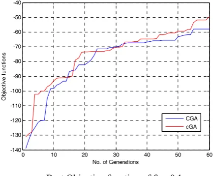
From Figure 3 and 4 it is clear that the quality of solutions and convergence speed found by the cGA is better than the CGA. The results suggest that the cGA performs the best and the CGA performs the worst.

0 10 20 30 40 50 60

-140 -130 -120 -110 -100 -90 -80 -70 -60 -50 -40

No. of Generations

O

b

je

c

ti

v

e f

u

n

c

ti

ons

CGA cGA

0 10 20 30 40 50 60

-180 -160 -140 -120 -100 -80 -60 -40

No. of Generations

O

b

je

c

tiv

e

F

u

n

c

ti

o

n

s

CGA cGA

0 10 20 30 40 50 60

-140 -130 -120 -110 -100 -90 -80 -70 -60 -50 -40

No. of Generations

O

b

je

c

tiv

e

F

u

n

c

ti

o

n

s

CGA cGA

Sample Size (n)

ࣂ૚ CGA cGA

F PSS F PSS

25

0.1 3200 9.7656 124 0.3784 -0.1 4150 12.6647 130 0.3967

0.4 3000 9.1552 116 0.3540 -0.4 3750 11.4440 124 0.3784

0.7 3400 10.3759 138 0.4211 -0.7 3900 11.9018 140 0.4272

50

0.1 3200 9.7656 122 0.3723 -0.1 3650 11.1389 126 0.3845

0.4 2800 8.54492 100 0.3051 -0.4 3500 10.6811 120 0.3662

0.7 3250 9.9182 128 0.3906 -0.7 3350 10.2233 120 0.3662

100

0.1 2250 6.8664 96 0.2929 -0.1 3000 9.1552 106 0.3234

0.4 2450 7.4768 98 0.2990 -0.4 3250 9.9182 116 0.3540

0.7 2650 8.0871 102 0.3112 -0.7 2850 8.6975 110 0.3356

-b- Best Objective function of

-a- Best Objective function of

-c- Best Objective function of ߠ_ଵ= 0.7

Figure 3. Results of best objective function (squared Error) of 60 generations over 5 Runs with n =25

V. CONCLUSION

In this paper, we investigate the performance of the compact Genetic Algorithm cGA for estimating the parameter of log-likelihood function ݈݊൫ܮሺߠǡ ߪ_௔ଶሻ൯of first order moving average model MA(1). Based on MSE, cGA provides effective results for three random samples with different sizes (n= 25, 50, 100) and ߠ is set to (טͲǤͳǡ טͲǤͶǡ טͲǤ͹) in comparison with the CGA and Moment Method. Simulation results show that the cGA has a higher optimal precision or at least the same as that obtained from the CGA, at same time, the cGA needs minimum searched space percentage and less number of function evaluations than that of the CGA.

REFERENCES

[1] E. Goldberg David, "Genetic algorithms in search, optimization and machine learning," Reprinted with corrections from Goldberg (1989) Addison Wesley Longman Inc, 1993.

[2] P. Larranaga and J. A. Lozano, Estimation of distribution algorithms: A new tool for evolutionary computation vol. 2: Springer Netherlands, 2002.

[3] M. Pelikan, et al., "A survey of optimization by building and using probabilistic models," Computational optimization and applications, vol. 21, pp. 5-20, 2002.

[4] R. Rastegar and A. Hariri, "A step forward in studying the compact genetic algorithm," Evolutionary computation, vol. 14, pp. 277-289, 2006

[5] S. Baluja, "Population-based incremental learning. a method for integrating genetic search based function optimization and competitive learning," DTIC Document1994.

[6] S. Baluja and R. Caruana, "Removing the genetics from the standard genetic algorithm," in The International Conference on Machine Learning 1995, 1995, pp. 38-46.

[7] G. R. Harik, et al., "The compact genetic algorithm," Evolutionary Computation, IEEE Transactions on, vol. 3, pp. 287-297, 1999.

[8] W. W. S. Wei, Time series analysis: Addison-Wesley Redwood City, California, 1990.

[9] B. Hussain and R. Al-Dabbagh, "A canonical genetic algorithm for likelihood estimator of first order moving average model parameter," NEURAL NETWORK WORLD, vol. 17, pp. 271, 2007.

[10] B. A. H. Al-Sarray, "Variants of Hybrid Genetic Algorithms for Optimizing Likelihood ARMA Model Function and Many of Problems," Evolutionary Algorithms, pp. 219-246, 2011.

[11] S. Droste, "A rigorous analysis of the compact genetic algorithm for linear functions," Natural Computing, vol. 5, pp. 257-283, 2006.

[12] I. J. Myung, "Tutorial on maximum likelihood estimation," Journal of Mathematical Psychology, vol. 47, pp. 90-100, 2003.

0 10 20 30 40 50 60

-700 -600 -500 -400 -300 -200 -100

No. of Generations

O

b

je

c

tiv

e

F

u

n

c

ti

o

n

CGA cGA

0 10 20 30 40 50 60

-650 -600 -550 -500 -450 -400 -350 -300 -250 -200 -150

No. of Gnerations

O

b

je

c

ti

v

e F

u

nc

ti

on

CGA cGA

0 10 20 30 40 50 60

-650 -600 -550 -500 -450 -400 -350 -300 -250 -200 -150

No. of Generations

O

b

je

c

tiv

e F

u

n

c

ti

o

n

CGA cGA

Figure 4. Results of best objective function (Squared Error) of 60 generations over 5 Runs with n = 100

-f- Best Objective function of ߠ_ଵ=െͲǤ͹ -d- Best Objective function of ߠ_ଵ= െͲǤͳ

[13] G. E. P. Box and G. M. Jenkins, Time series analysis: forecasting and control: Prentice Hall PTR, 1994.

[14] D. F. Chrysoula, "Yule-Walker Estimation for the Moving-Average Model," International Journal of Stochastic Analysis, vol. 2011, 2011.

[15] ] C. Aporntewan and P. Chongstitvatana, "A hardware implementation of the Compact Genetic Algorithm," in Evolutionary Computation, 2001. Proceedings of the 2001 Congress on, 2001, pp. 624-629 vol. 1.

[16] M. Spyros, et al., "Forecasting: Methods and Applications," ed: New York, USA: John Wiley & Sons Inc, 1997.