Wavelet Based Neural Networks for Daily Stream Flow Forecasting

(1)

International Journal of Emerging Technology and Advanced Engineering

Website: www.ijetae.com (ISSN 2250-2459,ISO 9001:2008 Certified Journal, Volume 4, Issue 1, January 2014)

307

Wavelet Based Neural Networks for Daily Stream Flow

Forecasting

Y. R. Satyaji Rao (Corresponding Author)

1

, B Krishna

2

, B. Venkatesh

3

1,2

Scientist, Deltaic Regional Center, National Institute of Hydrology, Kakinada-533 003, Andhra Pradesh, India 3_{Scientist, Hard Rock Regional Centre, National Institute of Hydrology, Hanuman Nagar, elgaum,}

Karnataka, India

Abstract--Unlike other hydrological time series data, rainfall and runoff time series data are highly variable spatially and temporally. However, stream flow measuring point is fixed in a river, therefore mapping of temporal variability of runoff can be handled with suitable algorithms. Time series analysis requires mapping complex relationships between input(s) and output(s), because the forecasted values are mapped as a function of patterns observed in the past. In order to improve the precision of the forecasts, a Wavelet Neural Network (WNN) model, based on a combination of wavelet analysis and Artificial Neural Network (ANN), has been proposed. The WNN and ANN models have been applied to daily runoff in the West flowing Rivers of India. The calibration and validation performance of the models is evaluated with appropriate statistical indices. The results of daily runoff series modelling indicated that the performances of WNN models are more effective than the ANN models. Further, WNN model performance has been evaluated separately for Low, Medium and High runoff values and found that the selected model is suitable for various runoff patterns from a catchment.

Keywords-- Time series, ANN, WNN, Runoff, India

I. INTRODUCTION

Most time series modelling procedures fall within the framework of multivariate Auto Regressive Moving Average (ARMA) models. Traditionally, ARMA models have been widely used for modelling water resources time-series modelling (Maier et al., 1997). Time-series models are more practical than conceptual models because it is not essential to understand the internal structure of the physical processes that are taking place in the system being modelled. However, these models do not attempt to represent the nonlinear dynamics inherent in the hydrological process, and may not always perform well (Tokar et al., 1999). Presently nonlinear models such as neural networks are widely used for time series modelling. Artificial Neural Networks (ANN) models were widely used to overcome many difficulties in time series modelling of hydrological variables (ASCE Task Committee, 2000a,b).

However, it is also reported that ANN models are not very satisfactory in terms of precision because they consider only a few aspects of the behaviour of the time series (Wensheng, 2003).To raise the precision, a wavelet analysis has been used along with ANN. The advantage of the wavelet technique is that it provides a mathematical process for decomposing a signal into multiple levels of details and analysis. Wavelet analysis can effectively decompose signals into the main frequency components while also extracting local information of the time series. In recent years, wavelet theory has been introduced in the field of hydrology (Smith et al., 1998; Labat et al., 2000). Due to the similarity between wavelet decomposition and the single-hidden layer neural network, the idea of combining both wavelet and neural networks has resulted recently in formulation of the wavelet neural network, which has been used in various fields (Xiao et al., 2005).

In this paper, a Wavelet Neural Network (WNN) model, which is the combination of wavelet analysis and ANN, has been proposed for runoff time series modelling of four west-flowing rivers in India: the Kollur, Seethanadi, Varahi and Gowrihole rivers.

II. WAVELET ANALYSIS

(2)

International Journal of Emerging Technology and Advanced Engineering

308

Wavelets are strongly connected to such processes in that the same shapes repeat at different orders of magnitude. The ability of the wavelets to simultaneously localize a process in a time and scale domain results in representation of many dense matrices in a sparse form.

The discrete wavelet transform of a time series f(t) is defined as:

dt

a

b

t

f

a

b

a

f

(

,

)

1 

(

)

(

)



 







(1)

Where (t) is the basic wavelet with effective length (t) that is usually much shorter than the target time series f(t); a is the scale or dilation factor that determines the characteristic frequency so that its variation gives rise to a “spectrum”; and b is the translation in time so that its variation represents the “sliding” of the wavelet over f(t). The wavelet spectrum is thus customarily displayed in the time-frequency domain. For low scales, i.e. when |a| <<1, the wavelet function is very concentrated (shrunk, compressed) with frequency content mostly in the higher frequency bands. Inversely, when |a| >> 1, the wavelet is stretched and contains mostly low frequencies. For small scales, we obtain thus a more detailed view of the signal (also known as “higher resolution”) whereas for larger scales we obtain a more general view of the signal structure.

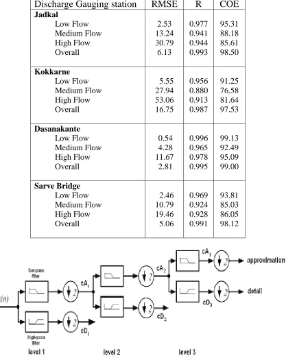
The original signal X(n) passes through two complementary filters (low pass and high pass filters) and emerges as two signals: approximations (A) and details (D). The approximations are the high-scale, low frequency components of the signal. The details are the low-scale, high frequency components. Normally, the low frequency content of the signal (approximation, A) is the most important. It demonstrates the signal identity. The high-frequency component (detail, D) is nuance. The decomposition process can be iterated, with successive approximations being decomposed in turn, so that one signal is broken down into many lower resolution components (Fig. 1).

Artificial neural networks

An ANN, can be defined as a system or mathematical model consisting of many nonlinear artificial neurons running in parallel, which can be generated as single or multiple layered. Although the concept of artificial neurons was first introduced by McCulloch & Pitts (1943), the major applications of ANNs have arisen only since the development of the back-propagation (BP) method of training by Rumelhart et al., (1986).

Following this development, ANN research has resulted in the successful solution of some complicated problems not easily solved by traditional modelling methods when the quality/quantity of data is very limited. ANN models are “black box” models with particular properties, which are greatly suited to dynamic nonlinear system modelling. The main advantage of this approach over traditional methods is that it does not require the complex nature of the underlying process under consideration to be explicitly described in mathematical form. ANN applications in hydrology vary, from real-time to event-based modelling.

Neural network structure

The most popular ANN architecture in hydrological modelling is the multilayer perceptron (MLP) trained with a BP algorithm (ASCE 2000a,b). A multilayer perceptron network consists of an input layer, one or more hidden layers of computation nodes, and an output layer. The number of input and output nodes is determined by the nature of the actual input and output variables. The number of hidden nodes, however, depends on the complexity of the mathematical nature of the problem, and is determined by the modeller, often by trial and error. The input signal propagates through the network in a forward direction, layer by layer. Each hidden and output node processes its input by multiplying each of its input values by a weight, summing the product and then passing the sum through a nonlinear transfer function to produce a result. For the training process, where weights are selected, the neural network uses the gradient descent method to modify the randomly selected weights of the nodes in response to the errors between the actual output values and the target values. This process is referred to as training or learning. It stops when the errors are minimized or another stopping criterion is met. The BPNN can be expressed as

Y = f (ΣW X – θ) (2)

Where X is the input or hidden node value; Y is the output value of the hidden or output node; f() is the transfer function; W is weights connecting the input to hidden, or hidden to output nodes; and θ is the bias (or threshold) for each node.

Methods of network training

(3)

International Journal of Emerging Technology and Advanced Engineering

309

In the ordinary gradient descent method, only the first-order derivatives are evaluated and the parameter change information is contained solely in the direction along which the cost is minimized. In practice, LM is faster and finds better optima for a variety of problems than most other methods (Hagan & Menhaj, 1994). The method also takes advantage of the internal recurrence to dynamically incorporate past experience in the training process (Coulibaly et al., 2000).

The Levenberg-Marquardt algorithm is given by:

Xk+1 = Xk –(JT J +  I)-1 JTe (3)

Where, X contains the weights of the neural network, J is the Jacobian matrix of the performance criteria to be minimized,  is a learning rate that controls the learning process and e is residual error vector.

If the scalar  is very large, the above expression approximates gradient descent with a small step size; while if it is very small; the above expression becomes the Gauss-Newton method using the approximate Hessian matrix. The Gauss-Newton method is faster and more accurate near an error minimum. Hence we decrease  after each successful step and increase it only when a step increases the error. Levenberg-Marquardt has large computational and memory requirements, and thus it can only be used in small networks (Maier & Dandy, 1998). However, it is faster and less easily trapped in local minima than other optimization algorithms (Coulibaly 2001a,b,c; Toth et al., 2000).

Selection of network architecture

Based on a physical knowledge of the problem and statistical analysis, different combinations of antecedent values of the time series were considered as input nodes. The output node is the time series data to be predicted in one step ahead. Time series data was standardized for zero mean and unit variation, and then normalized into the range [0 to 1]. The activation functions used for the hidden and output layer were logarithmic sigmoidal and pure linear function respectively. For deciding the optimal hidden neurons, a trial and error procedure was started with two hidden neurons initially, and the number of hidden neurons was increased up to 10 with a step size of 1 in each trial. For each set of hidden neurons, the network was trained in batch mode to minimize the mean square error at the output layer. To check for any over-fitting during training, a cross-validation was performed by keeping track of the efficiency of the fitted model. The training was stopped when there was no significant improvement in the efficiency, and the model was then tested for its generalization properties.

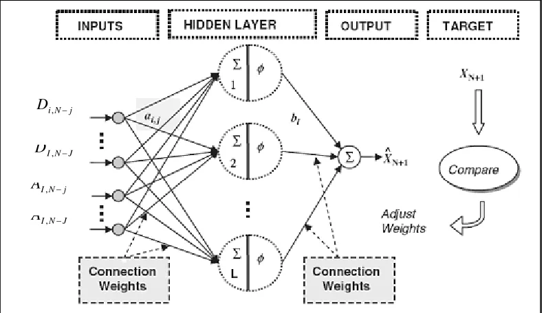
Figure 2 shows the multilayer perceptron neural network architecture when wavelet decomposed signal is used as the input to the neural network architecture.

Method of combining the Wavelet Analysis with ANN

The decomposed details (D) and approximation (A) are used as inputs to the neural network structure as shown in Fig. 2. Here, i is the level of decomposition varying from 1 to I, j is the number of antecedent values varying from 0 to J, and N is the length of the time series. To obtain the optimal weights (parameters) of the neural network structure, the LM algorithm is used to train the network. The output node represents the original value at one step ahead.

III. PERFORMANCE CRITERIA

The performance of various models (WNN and ANN) during calibration and validation were evaluated by using statistical indices: the root mean squared error (RMSE), correlation coefficient (R), and the Nash and Sutcliffe coefficient of efficiency (COE). RMSE measures the residual variance; which indicates a quantitative measure of the model error in units of the variable; the optimal value is 0. The correlation coefficient (R) measures the linear correlation between the observed and modelled values; the optimal value is 1.0. The COE, or efficiency (E%) compares the modelled and observed values and evaluates how far the network is able to explain total variance of data; the optimal value of COE is 1.0

IV. STUDY AREA AND DATA

(4)

International Journal of Emerging Technology and Advanced Engineering

310

Due to geographical conditions the measurement of daily rainfall and other climatic variables is difficult in densely forested basins and the availability of historical data is very limited.

V. RESULTS AND DISCUSSION

The daily runoff data of four west-flowing river basins namely Kollur, Sithanadi, Varahi and Gowrihole for the total period of 1981–2002 (22 years), 1973–1998 (26 years), 1978–2003 (26 years), and 1979–2003 (25 years) respectively is used for time series modelling. The daily runoff data of these four basins for the period of 1981– 1995 (15 years), 1973–1990 (18 years), 1978–1995 (18 years), and 1979–1995 (17 years) are used for calibration and for periods of 1996–2002 (7 years), 1991–1998 (8 years), 1996–2003 (8 years) and 1996–2003 (8 years) are used for validation period, respectively. The model inputs for each WNN model are indicated in Table 1 and the model inputs for each ANN model given in Table 2.

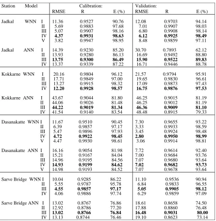
A total of five sub models were developed for each basin and these models were calibrated and tested for daily runoff series data modelling. The performance of these models in terms of global statistical tests (RMSE, R and %E) are given in Table 3. Similarly, five ANN models have been developed for four basins for the same period in which WNN models are developed. The performance of the ANN models in terms of global statistics are shown in Table 3.

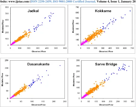
Table 3 reveals that the RMSE is much better (2.8 to 21.57 m3/s) for WNN models as compared to ANN (7.00 to 48.48 m3/s) models in all four basins during the validation period. From Table 3, it was also observed that among different antecedent values of the time series models (WNN), the model marked with bold shows lowest RMSE (2.8 to 16.75 m3/s), high correlation coefficient (0.9876 to 0.9950) and highest efficiency (97.53 to 98.99%) during the validation period in all four basins. Therefore, the WNN model (bold in Table 3) is selected as the best-fit model as compared to the ANN model to forecast the runoff in the rivers. Figure 3 shows the scatter plot between the observed and modelled values of WNN and ANN for four stations and shows that the forecast of daily runoff from WNN models were close to the measured values. Further, the measured runoff time series data in four basins have been classified into three categories (Low, Medium and High) using clustering technique. The details of each cluster (number of runoff values, mean, standard deviation, skewness) for observed and modeled runoff values are given in Table 4.

The mean values of observed runoff in low, medium and high flows are close to the mean value of modeled runoff values. The selected WNN model performance for each cluster interims of global statistics (RMSE, R and COE) are given in Table 5. The over all RMSE, R and COE for four basins indicated that the performance of selected WNN model is better than low, medium and high flows performance separately. However, it is always recommended to evaluate model performance for low, medium and high flows separately. The performance of WNN model (RMSE, R, COE) is better in low, medium and high flows consistently in Dasanakante gauging station. It may be due to the similar characteristics of runoff time series data during calibration and validation. The range of RMSE in four basins low, medium and high flows are (0.54 to 2.46), (4.28 to 27.94) and (11.67 to 53.06) respectively. Similarly, R-values are (0.958 to 0.996), (0.880 to 0.965) and (0.913 to 0.978) respectively. The COE ranges in low, medium and high flows are (91.25 to 99.13), (76.58 to 92.49) and (81.64 to 95.09) respectively. Further, the scatter plot between observed and modeled runoff values for each cluster (low, medium and high flows) is shown in Figure 4. Thus indicates the performance of WNN model is acceptable in all ranges of runoff time series modeling in the West flowing rivers.

VI. CONCLUSIONS

This paper has reported on an application of wavelet neural network (WNN) models for time series modelling of daily runoff of four west flowing rivers in India. Further, ANN models were also developed and the results are compared with WNN models. The comparison revealed that the WNN model exhibits better performance in modelling daily runoff time series data. Further, the WNN model performance was evaluated for low, medium and high runoff values separately during validation period and found that the selected WNN model can be used for all ranges of runoff. This is mainly due to the capability of wavelets to decompose the time series into multi-levels of approximation and detail. The models developed for runoff time series modelling would be useful for water resources planning in the Western Ghats where the measured runoff data availability is limited.

Acknowledgements

(5)

International Journal of Emerging Technology and Advanced Engineering

311

REFERENCES

[1] ASCE Task Committee (2000a) Artificial neural networks in hydrology-I: Preliminary concepts. J. Hydrologic EngngASCE 5(2), 115–123.

[2] ASCE Task Committee (2000b) Artificial neural networks in hydrology-II: Hydrologic applications. J. Hydrologic EngngASCE 5(2), 124–137.

[3] Coulibaly, P., Anctil, F., Aravena, R. & Bobee, B. (2001a) Artificial neural network modelling of water table depth fluctuations. Water Resour. Res. 37(4), 885–896.

[4] Coulibaly, P., Anctil, F. & Bobee, B. (2001b) Multivariate reservoir inflow forecasting using temporal neural network. J. Hydrologic EngngASCE 6(5), 367–376.

[5] Coulibaly, P., Anctil, F., Rasmussen, P. & Bobee, B. (2000) A recurrent neural networks approach using indices of low-frequency climatic variability to forecast regional annual runoff. Hydrol. Processes14, 2755–2777.

[6] Coulibaly, P., Bobee, B. & Anctil, F. (2001c) Improving extreme hydrologic events forecasting using a new criterion for ANN selection. Hydrol. Processes 15, 1533–1536.

[7] Hagan, M. T. & Menhaj, M. B. (1994) Training feed forward networks with Marquardt algorithm. IEEE Trans. Neural Networks 5, 989–993.

[8] Labat, D., Ababou, R. & Mangin, A. (2000) Rainfall–runoff relations for karstic springs: Part II. Continuous wavelet and discrete orthogonal multiresolution analyses. J. Hydrol.238, 149–178.

[9] Maier, H. R. & Dandy, G. C.(1997) Determining inputs for neural network models of multivariate time series. Microcomputers in Civil Engineering12, 353–368.

[10] Maier, H. R. & Dandy, G. C. (1998). Understanding the behavior and optimizing the performance of back-propagation neural networks: an empirical study. Environ. Modelling and Software 13, 179–191.

[11] McCulloch, W. & Pitts, W. (1943) A logical calculus of the ideas immanent in nervous activity. Bull. Mathematical Biophysics 5, 115–133.

[12] Rumelhart, D. E., Hinton, G. E. & Williams, R. J. (1986) Learning representations by back-propagating errors. Nature 323, 533–536 [13] Smith, L. C., Turcotte, D. & Isacks, B. L.(1998) Streamflow

characterization and feature detection using a discrete wavelet transform. Hydrol. Processes12, 233–249.

[14] Tokar, A. S. & Johnson, P. A. (1999) Rainfall runoff modelling using artificial neural network. J. Hydrologic Engng ASCE 4(3), 232–239.

[15] Toth, E., Brath, A. & Montanari, A. (2000) Comparison of short-term rainfall prediction models for real-time flood forecasting. J. Hydrol.239, 132–147.

[16] Wensheng, W. & Jing, D. (2003) Wavelet network model and its application to the prediction of hydrology. Nature and Science1(1), 67–71.

[17] Xiao, F., Gao, X., Cao, C. & Zhang, J. (2005) Short-term prediction on parameter-varying systems by multiwavelets neural network.

Lecture Notes in Computer Science (LNCS) no. 3611, 139–146. Springer-Verlag, Berlin, Germany.

Table 1

Model inputs for WNN model.

Model I Q(t)=f (x[t-1]) Model II Q(t)=f (x[t-1], x[t-2]) Model III Q(t)=f (x[t-1], x[t-2], x[t-3]) Model IV Q(t)=f (x[t-1], x[t-2], x[t-3], x[t-4])

Model V Q(t)=f (x[t-1], x[t-2], x[t-3], x[t-4], x[t-5])

Q(t) is daily runoff; f(x( )) is decomposed series of runoff

Table 2

Model inputs for ANN model.

Model I Q(t)=f (Q[t-1])

Model II Q(t)=f (Q[t-1], Q[t-2]) Model III Q(t)=f (Q[t-1], Q[t-2], Q[t-3]) Model IV Q(t)=f (Q[t-1], Q[t-2], Q[t-3], Q[t-4])

Model V Q(t)=f (Q[t-1], Q[t-2], Q[t-3], Q[t-4], Q[t-5])

(6)

International Journal of Emerging Technology and Advanced Engineering

[image:6.612.86.531.154.609.2]

312

Table 3

Performance of WNN and ANN models during calibration and validation.

Station Model Calibration:

RMSE R E (%)

Validation:

RMSE R E (%)

Jadkal WNN I II III IV V

Jadkal ANN I II III IV

11.36 0.9527 90.76 5.69 0.9883 97.68 5.07 0.9907 98.16 4.37 0.9931 98.63 3.82 0.9947 98.95

14.39 0.9230 85.20 13.93 0.9280 86.13 13.75 0.9300 86.49 13.37 0.9339 87.22

12.08 0.9703 94.14 7.01 0.9907 98.03 6.80 0.9908 98.14 6.12 0.9925 98.49 8.48 0.9859 97.11

30.70 0.7893 62.12 16.69 0.9492 88.80 15.90 0.9522 89.83 16.71 0.9446 88.78

Kokkarne WNN I II III IV

Kokkarne ANN I II III IV

20.16 0.9804 96.12 17.71 0.9849 97.00 13.27 0.9915 98.32 12.20 0.9928 98.57

43.67 0.9044 81.80 44.06 0.9026 81.48 44.22 0.9019 81.34 41.54 0.9140 83.54

21.57 0.9794 95.91 19.65 0.9830 96.61 17.09 0.9873 97.43 16.75 0.9876 97.53

46.25 0.9015 81.19 46.25 0.9012 81.19 46.36 0.9009 81.10 48.48 0.8915 79.33

Dasanakatte WNN I II III IV V

Dasanakatte ANN I II III IV

V

11.67 0.9510 90.45 6.39 0.9857 97.17 5.47 0.9896 97.93 4.72 0.9922 98.45 4.47 0.9930 98.61

16.16 0.9054 81.98 15.21 0.9167 84.04 14.96 0.9195 84.56 14.93 0.9199 84.62 14.98 0.9193 84.52

7.30 0.9655 93.22 3.33 0.9933 98.59 3.45 0.9924 98.48 2.80 0.9950 98.99 3.06 0.9914 98.81

7.72 0.9614 92.40 7.00 0.9684 93.76 7.07 0.9680 93.64 7.02 0.9682 93.73 7.07 0.9678 93.64

Sarve Bridge WNNI II III IV

Sarve Bridge ANN I II III IV

10.04 0.9285 86.22 5.55 0.9787 95.78 4.55 0.9857 97.17 4.06 0.9886 97.74

13.02 0.8767 76.86 12.92 0.8786 77.20 13.02 0.8766 76.84 13.13 0.8744 76.46

11.10 0.9536 90.94 6.84 0.9833 96.55 5.05 0.9905 98.12 6.29 0.9859 97.09

(7)

International Journal of Emerging Technology and Advanced Engineering

[image:7.612.74.541.167.494.2]

313

Table 4.

Critical analysis of selected WNN model performance in each cluster (Low, Medium and High) during validation period

Station

(Number of

daily flows)

Mean

Observed

Modeled

Standard Deviation

Observed Modeled

Skewness

Observed Modeled

Jadkal

Low Flow (2229)

Medium Flow (286)

High Flow (33)

Over all (2548)

7.51

99.41

334.81

22.06

7.58

98.72

337.84

22.08

11.67

38.58

82.44

49.95

11.84

38.85

93.01

50.35

2.05

0.96

0.24

4.57

2.13

0.95

0.47

4.75 Kokkarne

Low Flow (2337)

Medium Flow (442)

High Flow (33)

Over all (2922)

9.97

163.53

418.37

53.18

10.48

162.57

417.17

53.38

18.80

57.82

124.31

106.78

18.91

56.70

130.49

106.55

2.44

0.57

1.79

3.02

2.34

0.50

1.96

3.10 Dasanakante

Low Flow (2270)

Medium Flow (452)

High Flow (93)

Over all (2922)

3.93

38.07

132.14

13.47

3.97

38.69

128.33

13.49

5.75

15.63

52.93

27.97

5.83

16.14

51.42

27.47

1.44

0.92

1.69

4.58

1.44

0.98

1.86

4.65 Sarve Bridge

Low Flow (2270)

Medium Flow (386)

High Flow (39)

Over all (2925)

(8)

International Journal of Emerging Technology and Advanced Engineering

[image:8.612.136.524.169.683.2]

314

Table 5.

Selected WNN Model performance interims of global statistic indices in each cluster (Low, Medium and High) during validation

Discharge Gauging station

RMSE

R

COE

Jadkal

Low Flow

Medium Flow

High Flow

Overall

2.53

13.24

30.79

6.13

0.977

0.941

0.944

0.993

95.31

88.18

85.61

98.50 Kokkarne

Low Flow

Medium Flow

High Flow

Overall

5.55

27.94

53.06

16.75

0.956

0.880

0.913

0.987

91.25

76.58

81.64

97.53 Dasanakante

Low Flow

Medium Flow

High Flow

Overall

0.54

4.28

11.67

2.81

0.996

0.965

0.978

0.995

99.13

92.49

95.09

99.00 Sarve Bridge

Low Flow

Medium Flow

High Flow

Overall

2.46

10.79

19.46

5.06

0.969

0.924

0.928

0.991

93.81

85.03

86.05

98.12

[image:8.612.105.522.172.694.2]

(9)

International Journal of Emerging Technology and Advanced Engineering

[image:9.612.112.509.148.376.2]

315

Fig. 2 Wavelet based Multilayer Perceptron Neural network structure.

j N i

D

_, _

J N I

D

_, _

j N I

A

_, _

J N I

(10)

International Journal of Emerging Technology and Advanced Engineering

(11)

International Journal of Emerging Technology and Advanced Engineering

[image:11.612.82.531.120.473.2]