Efficient and compact representations of head related transfer functions

(1)

Efficient and Compact

Representations of Head Related

Transfer Functions

Author:

Joseph

_Sinker

Supervisors:

Prof. J.

_Angus

Prof. T.

_Cox

@00233333

School of Computing, Science, and Engineering

College of Science and Technology

University of Salford, Salford, UK

Submitted in Partial Fulfilment of the Requirements of the Degree of

(2)

List of Figures

2.1.1 Spatial cue formation . . . 5

2.1.2 Cone of Confusion . . . 7

2.2.1 Binaural recording . . . 9

2.4.1 A typical HRIR . . . 12

3.1.1 TU Berlin measurement scheme . . . 34

3.1.2 Measured HRIRs for cardinal directions with respect to left ear . . . 35

3.1.3 Measured HRIRs . . . 37

3.1.4 Measured HRTFs . . . 38

3.1.5 EDCs of ipsilateral and contralateral positions . . . 39

3.2.1 Comparison of ITD extraction methods . . . 41

3.3.1 Comparison of logarithmic and linear MSE calculations . . . 47

3.3.2 Comparison of maximum and minimum MSElin cases . . . 49

4.1.1 Linear magnitude basis vectors . . . 53

4.1.2 Linear magnitude weight vectors . . . 54

4.1.3 Pareto plot : Linear magnitude PCA . . . 56

4.1.4 Minimum reconstructed values of linear magnitude PCA . . . 58

4.1.5 Minimum reconstructed values against number of PCs used in reconstruction 59 4.2.1 Logarithmic magnitude basis vectors . . . 60

4.2.2 Logarithmic magnitude weight vectors . . . 62

4.2.3 Pareto plot : Logarithmic magnitude PCA . . . 63

4.2.4 Normalised mean squared error of 6 PC reconstruction . . . 64

(5)

J. Sinker Compact HRTFs LIST OF FIGURES

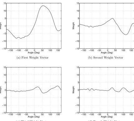
4.3.1 Basis vectors of first weight vector decomposition . . . 68

4.3.2 DCT representations of first PCA-1 weight vector . . . 71

4.3.3 DCT reconstruction of first weight vector . . . 72

4.3.4 Number of DCT components vs principal component weight vector order . . 73

4.3.5 DCT interpolation performance in MSE . . . 76

5.1.1 LPC diagram . . . 81

5.1.2 NMSE of all-pole model order 15 . . . 86

5.1.3 Maximum and minimum error HRTFs : All-pole order 15 . . . 87

5.1.4 MNMSE of all-pole model orders 1 to 100 . . . 88

5.1.5 Prior maximum and minimum error HRTFs of all-pole order 15 modelled with all-pole order 100 . . . 89

5.2.1 Lattice filter structure . . . 90

5.2.2 First 5 K coefficients variation with angle . . . 91

5.2.3 DCT reconstruction of first K coefficient across measured angles . . . 92

5.2.4 Number of DCT components vs K coefficient order . . . 93

5.2.5 NMSE performance of order 15 all-pole model using DCT approximation of K coefficents . . . 94

5.3.1 Simple linear problem . . . 95

5.3.2 Complex non-linear problem . . . 96

5.3.3 Iterative method system . . . 97

5.3.4 NMSE performance of 15 pole 15 zero model . . . 99

5.3.5 Measured and modelled spectra at angles of worst and best performance . . 100

5.3.6 Mean normalised mean squared error . . . 101

6.2.1 DT770 Pro frequency response [Man and Reiss, 2013] . . . 108

6.4.1 Histograms of reported positional differences per model . . . 112

6.4.2 Sigma of reported positional differences against model case . . . 113

6.4.3 Multiple comparison of model means . . . 115

(6)

Acknowledgements:

Firstly, I would like to thank Prof. Jamie Angus for her continued support and guidance throughout the project; allowing sufficient room for me to make progression through my own critical analysis whilst ensuring I did not stray too far from the path to completion.

Secondly, I would like to thank Prof. Trevor Cox, whose input throughout the length of the project was invaluable.

Thirdly, I would like to thank my fellow postgraduate students, who have acted as a sound-ing board, offersound-ing valuable suggestions and criticism throughout the project.

(7)

Abstract

These days most reproduced sound is consumed using portable devices and headphones, on which spatial binaural audio can be conveniently presented. One way of converting from conventional loudspeaker formats to binaural format is through the use of Head Related Transfer Functions (HRTFs), but head-tracking is also necessary to obtain a satisfactory externalisation of the simulated sound field. Typically a large HRTF dataset is required in order to provide enough measurements for a continuous virtual auditory space to be achieved through simple linear interpolation, or similar.

This work describes an investigation into the use of alternative compact and efficient rep-resentations of an HRTF dataset measured in the azimuthal plane. The two main prongs of investigation are the use of orthogonal transformations in a decompositional approach, and parametric modelling approach that utilises techniques often associated with speech processing. The latter approach is explored through the application of a linear prediction derived all-pole model method and a pole-zero model design method proposed by Steiglitz and McBride [Steiglitz and McBride, 1965]. The all-pole model is deemed to offer superior performance in matching the measured data after compression of the HRTF set through com-puter simulation results, whilst a preliminary subjective validation of the pole-zero models, that contrary to theoretical driven expectations, performed considerably worse in computer simulation experiments, is conducted as a pilot study.

(8)

Chapter 1 Introduction

The general public listen to audio and spatial audio content in a variety of ways; some-times this listening occurs in the home using traditional stereo or multi-channel loudspeaker setups. However, a large amount of this content is consumed on portable media devices such as smartphones, tablets, and digital media players, all of which commonly deliver au-dio content over headphones. Headphone listening may well account for a majority of the listening experience of many users. This trend is echoed by the recent decisions of major broadcast companies to move some traditional television and radio programming to online only platforms, clearly illustrating a reliable and foreseeably sustainable demand for content accessible from devices other than the traditional television or kitchen radio. Therefore, there is an increasing, and urgent, need to create effective and immersive experiences for headphone listeners utilising a wide range of devices.

(9)

J. Sinker Compact HRTFs CHAPTER 1. INTRODUCTION

ever falling cost of enabling software and technologies, and that lack the typically necessary equipment to trial audio material across multiple or even a single correctly realised repro-duction system(s).

Stereo headphones present a convenient and well realised platform for the delivery of spa-tial audio content. Headphones lend themselves particularly well to portability and use in multi-person environments. The acoustic signature of a listening environment, or a specific loudspeaker setup, is characterised by the relationship of the sound incident on each of a listener’s two ears from each of the sound sources present in the auditory space. Head-related transfer functions (HRTFs), describe the associated acoustic signal incident on each ear as a function of source location. Using a set of HRTFs measured at a specific listener’s ears, at the ears of a generalised mannequin of a head and possibly torso, or even via consideration of an analytical head model such as a sphere, positional cues can be synthesised for any number of discrete audio signals. As is imposed by the physical form of a pair of headphones, the resulting audio scene is reproduced through two discrete channels, feeding directly into the left and right ears individually. Commonly referred to as Binaural Stereo, this technique is the only effective method of rendering spatial audio content to a listener wearing headphones.

Binaural stereo audio is a well documented spatial audio technique, with implementations on a wide range of systems and devices. However, the majority of current implementations make use of large databanks of head-related transfer functions or head-related impulse re-sponses, in order to represent the auditory space around a listener’s head in as much detail as possible. For each possible location for which a sound can be synthesised, a pair of HRTFs or corresponding head related impulse responses (HRIRs) must be stored. Considering that HRIRs are commonly between 256 and 2048 samples long, it is clear that for accurate repro-duction purposes, a large number of HRTF/HRIR elements must be stored within the system.

(10)

J. Sinker Compact HRTFs CHAPTER 1. INTRODUCTION

The works described in this thesis comprise of an investigative exploration of techniques that can be used to achieve a more efficient means of ’handling’ the HRTF data required to achieve adequate coverage of a virtual auditory space. Previous approaches are broken down into three main categories; decompositional, filter modelling, and interpolation led, and are discussed at some length. Following discussion, the thesis presents and discusses the results and implications of the application, and in some instances, the extension of a decomposi-tional approach and two filter modelling approaches applied to a set of HRIR measurements made in the azimuth plane. Objective analysis is performed for all three methods through simulation of results with a subjective analysis of the most promising of the three methods conducted in parallel.

(11)

Chapter 2 Literature Review

A broad spectrum of works have already been conducted in the field of head-related transfer functions and their optimal representations, however the ongoing efforts of many authors to develop new methods tells that the question of efficient HRTF representation is still an open one. Past works have approached the problem from various angles but are commonly led by either the aim to compress the HRTF by some means, or alternatively to employ a robust means of HRTF interpolation. This section will attempt to summarise previous works on the topic, beginning with a brief introduction to the concept of the HRTF, then progressing to highlight important commonalities and differences in the methods and works of previous authors in the field that will go on to steadily influence the investigative works described in the latter sections of this thesis.

2.1 Localisation Cues

Spatial audio is the general term for audio that manipulates psychoacoustic cues to give the illusion of virtual sound sources positioned three dimensionally round a listener’s head. Spatial audio can be realised through a variety of reproduction systems ranging from two channel systems such as a stereo loudspeaker setup or headphones, to high order ambisonics arrays with many tens of loudspeakers.

(12)

J. Sinker Compact HRTFs CHAPTER 2. LIT. REVIEW

pair of headphones, the only difference in terms of signal is the inclusion of a cross coupling network between the two loudspeakers and the listener, whereas in the case of the head-phones the two audio channels are presented discretely to each of the listener’s ears.

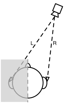
The localisation of a source within a space is a result of acoustic cues generated by the difference between a sounds arrival at each of a listener’s two independent ears. A listener’s ears are typically spaced between 18cm and 23cm apart, considering this spatial separation it is clear that the sound incident on each ear will differ depending on the ear’s proximity to the source and other factors [Howard and Angus, 2009].

[image:12.612.254.359.290.460.2]

L R

Figure 2.1.1: Spatial cue formation

2.1.1 ITD & ILD

(13)

be subject to a higher acoustic pressure due to the laws of spherical divergence, this effect is compounded by a more dominant effect; the ’acoustic shadow’ cast by the hard skull of the listener attenuating the sound incident on the occluded ear [Everest and Pohlman, 2009].

ITDs provide the dominant spatial cue for low frequencies below approximately 1500Hz [Z¨olzer, 2011]. Above this approximate limit the wavelength of sound is shorter than the spacing of the ears, subsequently the phase differences between the two ears become ambigu-ous and the ILD becomes the dominant cue.

Considering the case of the sound source positioned laterally at 90◦, i.e. at minimum dis-tance to one ear and maximum disdis-tance to the other, a rudimentary maximum value of the inter-aural time delay can be calculated as approximately 670µs, assuming a 23cm ear spacing [Woodworth, 1938].

2.1.2 Cone of Confusion

(14)

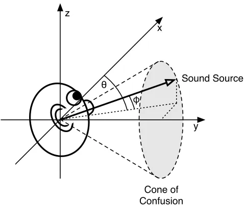
θ φ

Cone of Confusion

Sound Source z

x

[image:14.612.230.470.98.300.2]

y

Figure 2.1.2: Cone of Confusion

(15)

The second method of resolving directional ambiguities is the act of head movement, when a listener hears a sound of interest it is common for said listener to turn their head towards that sound, often attempting even to place the sound directly in front of the head at which the ITD and ILD cues will be equalised. The act of moving the head serves to alter the direction of sound arrival at the ears, this change in direction is dependent on the source position relative to the listener and will therefore serve to resolve the ambiguity. Movement of the head is an important factor to be considered in the attempted externalisation of binaural audio over headphones; if the auditory scene moves with the listener’s head then the listener is highly likely to lose the illusion of the audio emanating from elsewhere than the headphones themselves, this is referred to as internalisation. Systems can be designed to compensate the angle used as a criteria for HRTF selection in real-time by tracking the movement of the listener’s head by some means.

2.2 Binaural Stereo

(16)

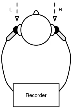
L R

[image:16.612.242.368.96.288.2]

Recorder

Figure 2.2.1: Binaural recording

Due to the naturally occurring variation in head and pinnae shapes between listener’s, indi-vidual listeners are accustomed to hearing a specific set of locational cues unique to them-selves. A binaural recording made with a specific head, be it real or artificial will achieve varying degrees of success of 3D reproduction across a multitude of listeners [Begault et al., 2001] [Wenzel et al., 1993].

2.3 Head-Related Transfer Functions

The Head Related Transfer Function (HRTF) describes the relationship between the sound emanating from a source in a spatial location and the sound incident at the open end of left or right ear canal (as specified). A pair of HRTFs, one for each ear, can be used to simulate sound emanating from the location described by the two HRTFs in question, as the HRTF encapsulates all of the ITD, ILD, filtering, and shading cues caused by reflections from the head, torso, and pinnae etc.

(17)

sine sweep may be used, as such the known stimulus signal must be deconvolved from the measured response at each ear to obtain the corresponding impulse response measurements.

HRTFs are often presented as twin sets of discrete responses representing a full, or sometimes limited, sweep of source angles around the head in both azimuth and elevation. Commonly denoted as HL(f, θ, φ) & HR(f, θ, φ) when presented in the frequency domain, where f

denotes frequency and θ and φ denote angle of azimuth and elevation respectively. The transfer functions are sometimes given in the time domain in the form of a Head Related Impulse Response, denoted as hL(t, θ, φ) & hR(t, θ, φ), where t denotes time. The HRTF

is simply the Fourier Transform of the HRIR, and thus the HRIR is the Inverse Fourier Transform of the HRTF.

2.4 Minimum Phase Assumption

Perhaps the best place to begin the analysis of the literature is with the discussion of the minimum phase assumption often adopted in an attempt to simplify the HRTF compression problem.

A system exhibits minimum phase characteristics if both the system and its inverse are causal and stable. In the z-domain this translates to the system having no poles or zeros on or outside the unit circle; poles outside the unit circle imply feedback gain of more than unity, hence the system would become unstable, zeros outside the unit circle, though stable in the original system, translate to unstable poles in the inverse of the system.

The inverse of a system H(z) can be thought of as a corresponding system H−1₍_z_{) that}

exactly rectifies the effect of the original filter, such that:

H(z)H−1(z) = 1 (2.4.1)

LettinghI(k) be the impulse response of inverse system H−1(z) in the discrete time domain

(18)

h(k)∗hI(k) = δ(k) =

  

0, k6= 0

1, k= 0

(2.4.2)

First presented by Mehrgardt & Mellert [Mehrgardt and Mellert, 1977], it was found that HRTFs can be approximated to be minimum phase systems. That is, the excess phase component that results from the subtraction of a minimum phase version of an HRTF from it’s original phase response has been shown to be approximately linear [Huopaniemi et al., 1999]. This minimum phase assumption implies that the HRTF can be decomposed into two sections [Oppenheim and Schaeffer, 1975]; the first is an angle-dependent frequency-independent delay line or all pass section, the second is the minimum phase filter section.

H(ejw) =Hap(ejw)Hmin(ejw) (2.4.3)

Where H is the HRTF, and Hap and Hmin are the associated all pass and minimum phase

components of H.

(19)

0 50 100 150 200 250 −0.8

−0.6 −0.4 −0.2 0 0.2 0.4 0.6 0.8

Samples

Amplitude

Figure 2.4.1: A typical HRIR

This assumption has been tested both objectively and subjectively, and deemed to have no significant undesired effects by several authors [Kistler and Wightman, 1992] [Kulkarni, 1995] [Kulkarni et al., 1999] [Nam et al., 2008].

The minimum phase assumption has been utilised in a wealth of works as it allows the excess delay component of the HRTFs, corresponding to the ITD, to be removed from consider-ation. The remaining minimum phase component of the HRTF is particularly convenient to work with as the minimum phase characteristic of the component implies that only the log-magnitude of the filter need be considered as the phase component is unique and obtain-able via the Hilbert transform of the log magnitude response [Kulkarni and Colburn, 2004] [Oppenheim and Schaeffer, 1975].

(20)

This removal of the need to preserve non-minimum phase information during the attempted transformation or modelling of HRTFs is an attractive property, however not all approaches have utilised this assumption. Chen. et al [1995] for example implement a means of HRTF compression considering the complex output of the Fourier transform of measured HRIRs, and Evans et al. [1998] perform a parallel analysis on both the magnitude and unwrapped phase components.

The works described in the latter sections of this thesis will adopt the minimum phase assumption of the HRTF, concentrating on the compression and efficient representation of the minimum phase component.

2.5 ITD Extraction

The topic of extraction of the interaural time differences from measured data follows closely from that of the minimum phase assumptions, as the ITD must be reintroduced to the mod-elled or compressed minimum phase component for synthesis. A number of different means of ITD extraction have been contrasted in prior works [Busson et al., 2005], [Lindau, 2010] [Minnaar and Plogsties, 2000].

It is noted by Mills [1958] that the threshold of detection for changes in ITD is approximately 10µsin optimal conditions. This fact must be taken into consideration as a common sample rate of 44100Hz has an inter-sample time step of approximately 23µs, subsequently it is pertinent in the interest of accurate ITD extraction to first upsample the measured impulse responses or use a peak detection scheme.

2.5.1 Spherical Head Model

(21)

IT Dθ = d

2c(θ+sinθ) (2.5.1)

Where d is the distance between the ears, often assumed to be 18cm, θ is the azimuthal angle, and cis the speed of sound.

This model is reasonably robust due to its physical nature, and gives a good approximation of the ITD in the azimuthal plane [Busson et al., 2005], however it is HRTF measurement independent, and will not provide accurate reproduction of individualised data.

2.5.2 IACC and IACCe Method

Presented by Kistler & Wightman [1992] the Inter-Aural Cross Correlation method models the ITD for a given angle as the time, or lag, for which the maximum value of the cross correlation function of the corresponding left and right ear impulse responses occurs. This approach is based upon the assumption that the auditory system utilises the cross correla-tion of signals present at the left and right ears in order to retrieve spatial informacorrela-tion and localise the sound source [Busson et al., 2005].

Minnaar & Plogsties report that the IACC method consistently overestimated the ITD by as much as 30µsapproaching the inter-aural axis [Minnaar and Plogsties, 2000], suggesting that the technique yields more accurate results if the left and right impulse responses are instead cross correlated with their respective minimum phase components. The ITD is then equal to the difference between the centroids of the left and right cross correlation functions.

Busson et al. suggest that the technique can be improved by instead computing the cross correlation of the signal envelopes of the corresponding left and right impulse responses for any given angle [Busson et al., 2005]. Dubbed the IACCe method, it was shown to perform well in perceptual testing.

(22)

impulse response and the possible lack of coherence between the ipsilateral and contralateral impulse responses for these angles [Busson et al., 2005].

2.5.3 Leading Edge Detection Method

Sandvad & Hammershøi propose a method for ITD extraction known as the Leading Edge Detection method, the ITD is calculated as the difference between the times at which each of the left and right impulse responses reaches a threshold value [Sandvad and Hammershoi, 1994]. The threshold value is defined separately for each of the left and right impulse re-sponses as a percentage of the peak value in the left and right impulse rere-sponses respectively. This method assumes that the initial portion of the HRIR consists purely of zeros after which the HRTF filter taps begin, i.e the min phase HRTF is preceded by a simple linear phase component.

Busson. et al found that this method successfully predicted the ITD the most closely when compared to psychoacoustic values alongside methods including the IACCe [Busson et al., 2005]. Somewhat conversely, Minnaar. et al remark that the method underestimates the ITD for angles between 90◦ and 110◦ [Minnaar and Plogsties, 2000], suggesting instead that it is appropriate when used in conjunction with a phase-based method to determine the inter-aural group delay of the excess phase components.

2.5.4 Phase Methods

Minnaar and Plogsties introduce a method of ITD extraction based upon phase analysis [Minnaar and Plogsties, 2000]. The ITD can be calculated by first evaluating the group delay of the excess phase component of the HRTF for each ear, the ITD is extracted as the inter-aural difference of the left and right group delay at 0Hz.

(23)

the other methods. They can however be made less reliable due to high-pass filtering effects introduced by the frequency response of measurement equipment [Estrella et al., 2010].

2.6 Decompositional Approach

An approach to achieving HRTF compression adopted by several authors is that which is based on the decomposition of the measured dataset into orthogonal subspaces. This can be achieved through the application of techniques commonplace in various disciplines such as the statistical Principal Component Analysis (PCA), the signal processing Karhunen-Loeve Theorem (KLT), or the image processing Singular Value Decomposition (SVD). All three techniques are built upon the efficient decomposition of data into a compressed, more efficient form, achieved through an orthogonal transformation. As such there exist applica-tions in which the three methods are interchangeable, but this is not true for all applicaapplica-tions.

The similarities and more importantly, the differences between the PCA, KLT, and SVD, are delineated in detail by Gerbrands [1981], who sought to alleviate the confusion surrounding the choice between the three techniques. Through detailed analysis of the three techniques it is revealed that in the case of a single vector or ann bymmatrix in which the mcolumns are regarded as m realisations of a random stochastic process that the PCA and KLT are in fact identical, apart from a possible shift of the coordinate system origin. If the column covariance matrix of the PCA and KLT is calculated from them realisations then the iden-tical PCA and KLT are also the same as the SVD, however this similarity only holds true in the application of the techniques to a single matrix [X] of m realisations. In the case of two-dimensional image processing, if the image [X] is considered to be a single realisation of a two-dimensional random process then the covariance matrices for the KLT and PCA techniques will be incorrectly calculated as they should be computed from a number of real-isations of that process, i.e. multiple images. It can be concluded that in the case of image processing the correct technique to be used is the deterministically defined SVD. For other applications concerning the realisations of a one dimensional random process the statistically defined PCA and KLT are appropriate.

(24)

multi-dimensional data set [Jolliffe, 2005]. Given a set of observations of possibly correlated variables, PCA transforms the data into a set of values in orthogonal basis referred to as principal components (PCs). The transformation is designed such that the first PC explains the largest amount of variance within the data set, the second PC explains the second largest amount of variance, and so on.

The output of the principal component analysis is the original data transformed into a series of basis vectors and associated weight vectors. The weight vectors describe the contribution of each of the basis vectors required to recreate the original data. Not only are the basis vectors an orthogonal series, but they are also uncorrelated with the weight vectors [Chen et al., 1995]; when considering an HRTF dataset this can be translated to the separation of frequency and angle. The basis vectors describe the principal spectral shapes in decreasing importance, and the weight vectors describe the variation in the basis vector contribution with respect to angle.

PCA attempts to convert a data set into its most efficient form, in which each subsequent component or variable contains only new information, this new information is always ac-countable for a smaller amount of total variance than that of the preceding component or variable.

The following equations detail the process of conducting a principal component analysis across the log magnitude spectra of an HRTF measurement suite [Kistler and Wightman, 1992]:

Firstly the log magnitude spectra are arranged in a matrix and empirical mean of the data is calculated:

uj = 1

n n

X

i=1

Xk,j (2.6.1)

Where uj is the mean spectrum,Xi,j is the matrix of the log magnitude spectra, and i and j are indexes such that Xk,j is an n by m matrix where k = 1,2, ...n and j = 1,2, ...m; n is

(25)

The mean is then subtracted from the original data:

Dk,j =Xk,j−uj (2.6.2)

In the case of an HRTF data set, the subtraction of the mean leaves a set of ’Directional Transfer Functions’ or DTFs. DTFs contain only information that is directionally unique, as artefacts common to all directional measurements, such as ear canal resonances, are removed with the subtraction of the ’mean spectrum’.

The next step is the computation of the covariance matrixS, where the covariance of a given pair of frequencies is defined as:

Si,j =

1

n(

X

Dk,iDk,j) (2.6.3)

for i, j = 1,2..., m

Where againnis the total number of transfer functions,mis the total number of frequencies, and Dk,i is the log magnitude at the ith frequency of the kth DTF.

The basis vectors are the eigenvectors of the covariance matrixS, the lowest ’order’ of which correspond to the largest eigenvalues,q.

The weights Wk corresponding to the contribution of each basis vector to a given DTF is

given by:

Wk =C0dk (2.6.4)

Where C is a matrix, of which the columns are the basis vectors and dk is the kth DTF

magnitude vector.

And hence the DTF magnitude vector is equal to a weighted sum of the basis vectors:

(26)

Once the analysis has been conducted the original data set can be fully reconstructed through a weighted sum of the total number of basis functions. However, a partial reconstruction of the original data can also be created from the weighted sums of any number of the low-est ’order’ principal components, this allows for a compromise between the total amount of original variance explained by the reconstruction, and the greatly reduced expression of the original data set. This was documented by Kistler & Wightman, who found that approxi-mately 90% of the variance of their 5300 HRTF dataset (2 ears of 10 subjects measured at 265 locations) could be expressed with a reconstruction based upon only the first 5 principal components [Kistler and Wightman, 1992]. Similar levels of compression have been achieved when the technique is extrapolated to much larger datasets, such as the CIPIC database of 56250 HRTF pairs (45 subjects measured at 1250 locations), for which Wang et al found that approximately 92% of the variance in the HRTF magnitudes was captured by the first 10 basis functions [Wang et al., 2008].

Chen et al [1995] applied similar techniques; utilising the discrete Karhunen-Loeve expan-sion to decompose the complex valued Fourier transform of measured HRIRs. The resulting complex valued eigentransfer functions (EFs) are a set of orthogonal frequency dependent functions, by projecting each EF onto the measured data the accompanying weight functions are derived. The weight functions are termed spatial characteristic functions (SCFs) as they are functions of only spatial location. 99.9% of the variance is captured by the first 12 EFs for the measured KEMAR data used in the work, though this is a larger number of basis vectors than was reported by Wightman & Kistler [1992], it is important to note that the technique proposed by Chen et al captures both the magnitude and phase components of the HRTFs.

(27)

a series of thin plate splines to fit the real and imaginary components of each of the Spa-tial Characteristic Functions derived from the decomposition of the complex valued Fourier components, whereas Carlile et al. opt to fit a series of spherical thin plate splines to the principal component weights derived from the decomposition of the frequency domain mag-nitude components of the HRTF dataset used.

Both studies found the interpolation to be reasonably robust; Chen et al. report average percent mean squared errors of less than 1% over most of the frontal and ipsilateral regions, with larger errors occurring in contralateral and lower elevation regions [Chen et al., 1995]. Carlile et al. conclude that by reducing the number of measurement positions retained in a series of models, all of which are constructed from a single measured superset of data, that a high fidelity recreation of a continuous auditory space can be achieved with as few as 150 evenly distributed recorded HRTF positions [Carlile et al., 2000].

The increased error of interpolated data at contralateral positions can be attributed to the large inter-aural level difference due to head shadowing [Chen et al., 1995].

(28)

Evans et al. conclude, similarly to the other authors mentioned in this section, that a large HRTF dataset can successfully be decomposed into a series of basis functions and correspond-ing weight functions, in this case a parallel pair of the first 17 surface spherical harmonics and their derived weight functions for both the magnitude and phase components [Evans et al., 1998]. However it is noted that although the surface spherical harmonic method proposed yields greater consistency in recreation of measured data, it does not perform as robustly as Chen et al’s EF and SCF based analysis when interpolation error is considered.

Comparatively, the surface spherical harmonic based decomposition does not offer as great an efficiency as other techniques mentioned in this section, however it is most appropriately compared to the approach proposed by Chen et al. [1995] as neither of these methods rely on the minimum phase assumption, opting instead to directly encode the phase in the pre-scribed methods. It is remarked by Evans et al. that for applications concerned with storage efficiency, the Karhunen-Loeve expansion based method proposed by Chen et al. may be considered more appropriate [Evans et al., 1998].

Like the surface spherical harmonic led approach proposed by Evans et al. [1998], Zhang et al. propose a decomposition approach not based on optimality such as the PCA and KLE approaches, but by instead using non-measurement specific functions with mathematical definition as the bases [Zhang, 2009]. A continuous two dimensional model of the azimuthal plane is constructed,a Fourier-Bessel series is used to reproduce the spectral variation in measured data, and a Fourier series is used in tandem to reproduce the corresponding spa-tial variation. Empirical data is used to guide the choice of orthonormal function as the basis function for the spectral variation, however even so, the basis functions are independent of the empirical data, and all subject or measurement dependent differences are encoded in the model coefficients. In validating the model, Zhang et al. directly compare their modelling technique to those previously conducted using the statistical based PCA [Kistler and Wight-man, 1992] and KLE [Chen et al., 1995] methods, by re-implementing them on the same 2D dataset.

(29)

components of the HRTFs [Zhang, 2009]. The KLE method is reported to give marginally superior error in the reconstruction of both the magnitude and phase data for a little over 300 less model parameters than the total of 4900 used in the proposed Fourier-Bessel / Fourier model. It is concluded that the proposed model’s measurement data independence and continuous nature, without the need for interpolation (spline fitting), is advantageous over the aforementioned KLE techniques.

The potential efficiency of the PCA based approach is furthered by Wang et al., who propose that following a PCA decomposition of the CIPIC HRTF database, the principal component weights may be expressed further more efficiently using a vector codebook technique [Wang et al., 2008]. The codebook technique achieves compression via a technique known as vector quantisation, in which a given vector is approximated by the nearest matching vector in a designed vector codebook, allowing the input vector to be recorded as a single value repre-senting the closest matching codebook index. Wang et al. report that the error introduced by the quantisation can be considered negligible; 7.23% compared to the 6.71% average error already present in the unquantised PCA reconstruction.

2.7 FIR and IIR Modelling

Another arm of approach to the problem of HRTF compression comes not from a basis of decomposition, but rather the consideration of the HRTF as an implementable digital filter.

The simplest of such implementations is to utilise the HRIR itself; the samples of a given HRIR, or any IR for that matter, represent the taps or coefficient weights of a finite impulse response (FIR) digital filter [Z¨olzer, 2011]. A rudimentary form of HRTF compression can be realised by truncating, or windowing, the measured HRIRs to reduce the number of filter taps, usually referred to as the order of the filter, used to represent each component of the HRTF dataset.

(30)

[Sandvad and Hammershoi, 1994], though rectangular windowing can result in frequency do-main oscillation or ripple known as the Gibbs phenomenon, the nature of the HRIR filters, more specifically their lack of frequency domain discontinuities, allows for simple rectangu-lar windowing to be used with negligible undesired effects being introduced to the frequency domain response of the filters. The use of alternative window designs, such as the Ham-ming window, typically selected as an alternative to rectangular windowing in an attempt to negate the influence of the Gibbs phenomenon, significantly smooths the frequency do-main response of the filter, which could possibly translate to the loss of pertinent spectral characteristics contained in the ’detail’ of the response.

Several authors have conducted works which suggest that the fine detail lost in HRTF smoothing or HRIR truncation is perceptually unimportant. Senova et al. [2002] found that the psychoacoustic performance of truncated HRIRs only began to perform poorer than free field loudspeaker signals for IR lengths of between 0.32 and 5.12ms. Through the use of a gammatone filterbank designed to mimic the spectral filtering of the human cochlea, Breebaart and Kohlrausch [2001] show that HRTF phase and magnitude spectra do not need a higher spectral resolution than that of the filterbank of the peripheral auditory system. More specifically they show that a first order gammatone filterbank with bandwidths of one equivalent rectangular band sufficiently describes the phase and magnitude spectra. In par-ticular the high frequency content of the HRTF has been shown to be of little importance for both the ipsilateral and contralateral ears, with the least detriment to psychoacoustic perception occurring for the contralateral Xie and Zhang [2010]. As such it can be con-sidered that the truncation of measured HRIRs may provide a simple means of reducing the number of stored elements in an HRTF/HRIR dataset without significantly altering the psychoacoustic perception of the data. Furthermore, simple HRIR truncation could be used in conjunction with further methods of compression to improve the overall efficiency of the system.

(31)

com-J. Sinker Compact HRTFs CHAPTER 2. LIT. REVIEW

paratively high order FIR implementations, in far fewer coefficients. This is due to the IIR filter’s feedback coefficients in the denominator of the transfer function, which can create a more pronounced response with superior efficiency to the FIR in terms of processing power required for implementation.

The IIR approximation of a given system, such as the HRTF for a given direction, can be derived by modelling the time domain system output, the HRIR, as the output of an auto-regressive moving average (ARMA) system [Farhang-Boroujeny, 1999]. For an ARMA system the output sample y(k) is defined as the weighted sum of all previous input and output samples, this can be expressed as:

y(k) = − n

X

i=1

aiy(k−i) + m

X

i=0

bix(k−i) (2.7.1)

and yields the transfer function:

H(z) =

m

P

i=0

biz−i n

P

i=0

aiz−i

= B(z)

A(z) (2.7.2)

Where x is the record of input samples, m and n are the orders of the numerator and de-nominator respectively, and ai and bi are the coefficients or tap weights.

The poles of the model, the locations of which are described by the denominator of the transfer function; the a coefficients, make up the auto-regressive component of the system, and in the case of the HRTF, translate to the acoustic resonances in the sound path be-tween the source and the ear. The zeros of the model, the locations of which are described by the numerator of the transfer function; the b coefficients, make up the moving-average component of the system, and in the case of the HRTF, translate to the anti-resonances and reflections in the sound path between the source and the ear [Asano et al., 1990].

(32)

between the model and the system to be modelled, first proposed by Kalman [Kalman, 1958]:

E2 = 1 2π

π

Z

−π

|H(w)A(w)−B(w)|2_dw _(2.7.3)

Where A(w) = A(z)|z=ejw and B(w) = B(z)|_z₌_ejw.

Kulkarni & Colburn detail two low order model approximations made using IIR filters; an all-pole model and a general pole-zero model [Kulkarni and Colburn, 2004]. The all pole case is derived as an implementation of the autocorrelation method for linear prediction as described by Makhoul [1975], whereas the pole-zero case is derived from a weighted-least-squares variation of the modified least-weighted-least-squares problem proposed by Kalman [1958]. The pole-zero derivation uses a technique known as the Steiglitz-McBride iteration [Steiglitz and McBride, 1965] to minimise the quadratic error function presented by Kalman, and obtain the optimum coefficients of the IIR filter model. In order to simplify the modelling process the mean spectrum was computed and subtracted from all HRTFs, thus leaving the DTFs, as described in the initial steps of the PCA procedure implemented by Wightman & Kistler [1992]. The removal of the mean, or common, spectral components of the data is believed to likely reduce the order of the derived IIR models needed to sufficiently recreate the measured dataset, as only the spatially dependent variances are encoded in such an approach. Small scale subjective evaluation across three subjects found that a model with just 6 poles and 6 zeros, was largely indistinguishable from original measurements, the 25 pole all-pole model performed similarly well but it does not provide as much representational efficiency as the pole-zero formulation.

(33)

Kulkarni & Colburn provide an insightful comparison into the differences in the approaches, and subsequently results, of the two studies. Asano et al. report that comparatively high model orders (40 poles and 40 zeros) were required to approach the same psychophysical per-formance as was found with the measured HRTFs in an absolute localisation task; clashing with the finding of Kulkarni & Colburn, that as low an order as 6 poles and 6 zeros is almost indistinguishable from the empirically obtained data. The difference in findings is explained as a combination of two likely sources of inconstancy between the studies. Firstly, the model proposed by Asano et al. is based on the Kalman estimate algorithm alone, whereas the method proposed by Kulkarni & Colburn utilises an iterative weighting procedure ([Steiglitz and McBride, 1965]) to achieve an optimal fit between the modelled and measured HRTF log magnitude functions. Secondly, Asano et al. modelled the HRTFs directly, whereas Kulkarni & Colburn modelled the DTFs calculated as the HRTFs of a dataset less the empirical mean. It is likely that the modelling of the more complex HRTFs that include not only the spatially dependent characteristics but the common-to-all spatial independent characteristics as well, means that the efficiency of the modelling process is reduced due to the need to fit poles and zeros to these addition spectral characteristics [Kulkarni and Colburn, 2004].

Ramos & Cobos present a parametric model of the HRTF based on a low order IIR imple-mentation achieved as a chain of second order sections of conventional shelving and peak audio filters [Ramos and Cobos, 2013]. The minimum phase component of the HRTF is modelled via an iterative process for which the central frequency wi, log-gain Gi, and the

quality factorQi of the shelving ad then successive peak filters is defined in order. A random

(34)

transformation of HRIR samples to 3-parameter filter section parameters, but that the filter parameters also represent a convenient means of performing a nearest neighbour interpola-tion scheme.

2.8 Interpolation Led Approaches

An alternative means of improving the efficiency of HRTF storage, or in particular the re-duction in measurement redundancy, such that less measurements need be performed, is to deduce a means of interpolating a dense measurement scheme from a comparatively sparse one.

Nishimura et al. propose an interpolation algorithm based upon spatial linear prediction [Nishimura et al., 2009]. The method requires that a single set of measurements are made with a high spatial resolution, this resolution defines the interpolation points for additional datasets. The high resolution data is used to calculate the optimum filter coefficientsw, that satisfy the system of simultaneous equations associated with the theory of linear prediction, against the complex Fourier coefficients of the HRTF set. The coefficients obtained can be used to interpolate HRTF sets measured at a lower spatial resolution as far as the limit im-posed by the spatial resolution of the dataset used to calculate the coefficients. The method attempts to exploit the observed periodicity of the measured HRTFs in the azimuthal plane, Nishimura et al. report a significant reduction in interpolation error compared to simple linear time domain alternative methods, as well as an increased rate of correct judgement of the rotation of a virtual sound source in unofficial listening tests. It is concluded that the interpolation method might be expanded by interpolating the coefficient set, which would allow interpolation of coarse datasets up to higher spatial resolutions than the current limit of the resolution of the dataset used to derive said coefficients.

(35)

same time domain interpolation with a correction to equalise impulse response arrival time, as was suggested as the outcome of investigation by Matsumoto & Yamanaka [2004]. The aforementioned investigation [Matsumoto and Yamanaka, 2004] considered the differences of accuracy of three interpolation methods, with and without arrival time correction. The ar-rival times of the interpolated responses were calculated linearly from the difference between the cross correlation of the left and right ear impulse responses for the two adjacent mea-sured angles. The methods considered were simple linear interpolation, spline interpolation, in which a piecewise mathematical polynomial is fitted to the data to achieve a continuous functional representation, and a method based on the Discrete Fourier Transform (DFT). The DFT method consists of arranging all HRIRs as the columns of a matrix and taking the DFT of each row, the output of each DFT is then transformed by adding zeros to the center of the array, finally the inverse DFT is taken of each of the transformed arrays resulting in a larger matrix of spatially oversampled HRIRs. Arrival time correction coupled with the simple linear interpolation case was shown to yield the greatest interpolation accuracy of the six cases for most angles, and arrival time correction improved the accuracy of all three methods, the results were assessed by comparing the signal to deviation ratio of the interpolated and measured HRIRs.

(36)

Due to the physical nature of the method in question [Duraiswaini, 2004], in particular the modelled source-encapsulating sphere, the scattering analysis method yields impressive re-sults when compared to the analytical model of a spherical head as used by Duda & Martens [Duda and Martens, 1998], the objective analysis of the scattering analysis model also fair well when fitted to a set of KEMAR data. The evolution of the predicted potential field at varying distances offers logical physical arguments including the growth of the HRTF magnitude in the direction corresponding to the direct path, and the enlargement of the shadowed magnitude region as the source approaches the head. It is noted that although highly promising, the reported results are based on objective analysis alone, and performance of the method should be investigated perceptually.

Some approaches to HRTF interpolation have been designed to take large numbers of, or even all of, the measurement points within a dataset; although such approaches have yielded increased interpolation accuracy over methods that consider only a small subset of measure-ment positions, they demand comparatively high computational expenses. This increased computational expense can become troublesome when attempting to render a complex au-ditory scene containing multiple sources, even more so if the sources are to be rendered as moving through the virtual auditory space.

A relatively straightforward approach to HRIR interpolation is to apply the bilinear inter-polation method; considering a subset of the four closest points for which measured data is available. Given an HRIR dataset containing information for all points on the measure-ment grid defined by the fixed angular intervals θgrid for azimuth and φgrid for elevation. An

interpolated HRIR for a desired direction (θ, φ) can be evaluated as:

hi(k) = (1−cθ)(1−cφ)ha(k) +cθ(1−cφ)hb(k) +cθcφhc(k) + (1−cθ)cφhd(k) (2.8.1)

whereha(k),hb(k),hc(k), andhd(k) are the HRIRs of the four adjacent measurement points,

and cθ and cφ are the normalised relative angular positions, calculated as:

cθ =

θ mod θgrid θgrid

cφ =

φ mod φgrid φgrid

(37)

Bilinear interpolation of four adjacent measurement points has been shown to exhibit smoother variation with change in angle than similar methods, such as bilinear interpolation of three adjacent measurement points [Gamper, 2013]. This property yields smoother interpolation, without discontinuities, and is an attractive facet in the rendering of moving sources.

Gamper proposes an alternative method of subset selection and subsequent interpolation based on the vectorisation of the HRTF measurement grid [Gamper, 2013]. Assuming a source distance of at least 1m for all measured points and desired points (to be interpolated), the distance effects of the HRTF can be assumed to be negligible, thus the directions to all measurement points and desired points can be described as unit vectors. Gamper’s proposed method is based on the assumption that an HRTF estimate for the desired source direction

s can be constructed as a linear combination of three measurement directionsh1, h2, h3 that

form an enclosing convexly curved triangle around s on the unit sphere. In the interests of both speed and computational efficiency a triangulation of the unit sphere is performed as the algorithm is initialised; during which the surface of the unit sphere is mapped as a series of non overlapping triangles constructed from triplets of measurement points, the results of which are stored. A Delaunay triangulation is used to maximise the minimum angle of all the angles of the triangles in the triangulation, this has been shown to be advantageous for interpolation by other authors. To further increase runtime efficiency, the inverse of each measurement point triplet, required to calculate the contribution gain of each measurement vector to obtain the desired direction, is calculated and stored during the same initialisation process.

(38)

2.9 Conclusion

It is evident from the literature discussed in this section that given an interest in both effi-cient representation and interpolation of the HRTF dataset then an interpolation led method is largely unsuitable, though an interpolation based approach can be thought of as offering a means of compression through the reduced number of measurements that need be stored this level of compression is minimal in comparison to that which is achievable via a decom-positional or filter modelling approach.

Both the decompositional and filter modelling approaches have apparent strengths and some similar weaknesses, such as the recurring increased error at contralateral positions, however no one method seems to be identifiable as optimal in so far as to offer maximal compression for minimal loss in reconstruction/model error. As such the experimental works described in this thesis will approach the initial compression problem from both a decompositional and parametric filter modelling standing. In order to take advantage of possible underlying cyclic features of the HRTF and also to simplify the problem to a more appropriate project length, the methods will be investigated using an HRTF dataset limited to the azimuthal plane only.

Restricting the analysis to the horizontal plane somewhat limits the exploration of spectral compression methods, as many of the psychoacoustically significant spectral variations are an effect of the influence of the asymmetrical pinnae on changes in source elevation. How-ever this limitation should not affect the objective analysis of the compression methods or interpolation scheme presented in the remainder of this work. Furthermore, human ability to detect source direction is known to be most acute in the horizontal plane as such it can be considered to be of principal interest, particularly in the context of interpolation.

(39)

(40)

Chapter 3 Preparation for Experimental Works

3.1 TU Berlin HRTF Analysis

This section of the report gives a brief analysis of the dataset used as the basis of the inves-tigative works described in the following sections. The aim of this section is to highlight the key features of the HRTF and HRIR in the azimuthal plane, and familiarise the reader with the measured dataset.

For this project, the HRIR measurement dataset chosen has been provided by TU Berlin [Wierstorf et al., 2011], the set is made freely available under a Creative Commons Attribution-NonCommercial-ShareAlike 3.0 license.

The impulse responses were measured in an anechoic chamber, with lower frequency limit 63Hz, using a KEMAR mannequin at a range of four different loudspeaker distances; 0.5m, 1m, 2m, and 3m. The excitation signal was a 5.3s linear sine sweep with a 6dB per octave low-shelf emphasis below 1kHz, resulting in an amplification of 20dB for low frequencies.

The loudspeaker was positioned at ear-level, and a high precision stepper motor was used to rotate the mannequin in order to obtain measurements in increments of one degree in the azimuthal plane.

(41)

J. Sinker Compact HRTFs CHAPTER 3. PREPARATION

the minimum ITDs were determined between measurement angles−90◦ and 90◦, the dataset was then rotated by 2◦−3◦ to align the minimum to 0◦, secondly the ILD between the two ears was corrected by adjusting the gain of the left and right HRIRs to achieve an ILD of 0dB at 0◦. The loudspeaker transfer function was also compensated between 100Hz and 10kHz by the design and application of inverse FIR filters.

θ

r= 0.5m, 1m, 2m, 3m

Figure 3.1.1: TU Berlin measurement scheme

(42)

0 50 100 150 200 250 −0.8 −0.6 −0.4 −0.2 0 0.2 0.4 0.6 0.8 Samples Amplitude

(a) 0◦: Front

(b)−90◦ : Contralateral

(c) ±180◦ : Rear

[image:42.612.83.522.118.503.2]

(d) 90◦ : Ipsilateral

Figure 3.1.2: Measured HRIRs for cardinal directions with respect to left ear

(43)

measurement positions are approximately equidistant from the either ear. Comparing subfig-ures 3.1.2b and 3.1.2d clearly conveys the difference in sound path between the contralateral and ipsilateral ear respectively. The ipsilateral position clearly yields maximal excitation out of the four cardinal directions, as well as the shortest onset/arrival time, conversely the contralateral position is characterised by minimal excitation due to the acoustic shading of the head positioned directly between the speaker and, in this case occluded, ear, and the longest onset/arrival time of all four pictured responses.

All four of the HRIRs presented in figure 3.1.2 share a common onset delay before the vari-able onset delay due to measurement position. The common onset delay occurs due to the distance between the loudspeaker and the dummy head used to measure the data; the data was measured with a constant distance of 1m between the centre of the loudspeaker and the centre of the mannequin. In post-processing the length of the onset delay of all 1m measurements was trimmed to that equivalent to a measurement distance of 0.5m between the centre of the loudspeaker and the centre of the mannequin [Wierstorf et al., 2011]. At the sample rate of 44100Hz a distance of 0.5m should correspond to a common onset delay of approximately 64 samples, however due to the distance from the centre of the mannequin to the microphone transducers at the ear canals, this value is slightly too large. A better estimate is to address the case of the ipsilateral measurement position; assuming an ear spacing of 0.18m, true of the KEMAR design, the expected onset delay due to measurement distance of (0.5-0.09) 0.41m is approximately 53 samples. This seems congruent with the measured impulse response of the ipsilateral position in subfigure 3.1.2d, which seemingly exhibits an onset delay of similar order to the approximated value.

(44)

Azimuth (Deg)

Sample N

o

−150 −100 −50 0 50 100 150 20 40 60 80 100 120 140 Sample Value −0.4 −0.2 0 0.2 0.4 0.6 0.8

(a) Left Ear

Azimuth (Deg)

Sample N

o

−150 −100 −50 0 50 100 150 20 40 60 80 100 120 140 Sample Value −0.4 −0.2 0 0.2 0.4 0.6 0.8

[image:44.612.81.536.109.298.2]

(b) Right Ear

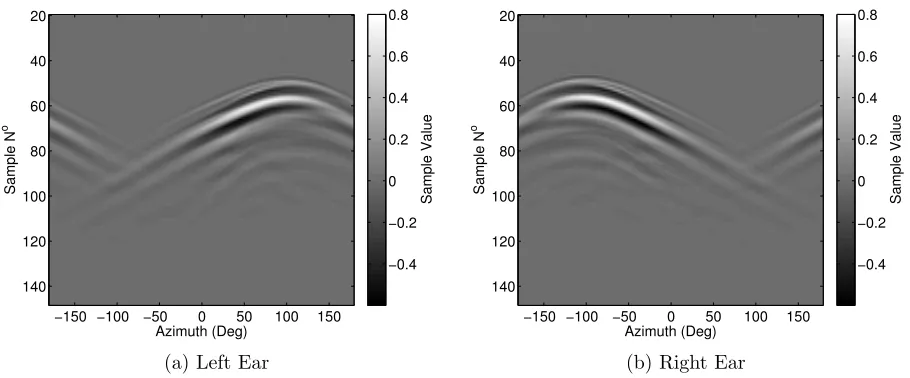
Figure 3.1.3: Measured HRIRs

Figure 3.1.3 shows a portion of the measured head related impulse responses for all measured angles at each ear. For illustrative purposes only 128 samples of the impulse responses have been plotted, starting at sample number 20 and ending with sample number 148. Both the inter-aural time and level differences can be seen clearly across the angular variation; the highest contrast areas represent maximal excitation in the measured sound field. It is evident that the largest amplitudes occur in the ipsilateral regions for each ear, occurring around +90◦ for the left ear in figure 3.1.3a and around−90◦ for the right ear in figure 3.1.3b. The image plots also show the variation in onset delay of the HRIRs with respect to the variation in source angle, the uppermost region of excitation on each of the two plots, corresponding to the shortest onset delay, occurs as expected at the ipsilateral source position of +90◦ and

(45)

Azimuth (Deg)

Frequency (Hz)

−150 −100 −50 0 50 100 150 0

0.5 1 1.5 2

x 104

Magnitude (dB) −80 −60 −40 −20 0 20

(a) Left Ear

Azimuth (Deg)

Frequency (Hz)

−150 −100 −50 0 50 100 150 0

0.5 1 1.5 2

x 104

Magnitude (dB) −80 −60 −40 −20 0 20

[image:45.612.85.532.106.298.2]

(b) Right Ear

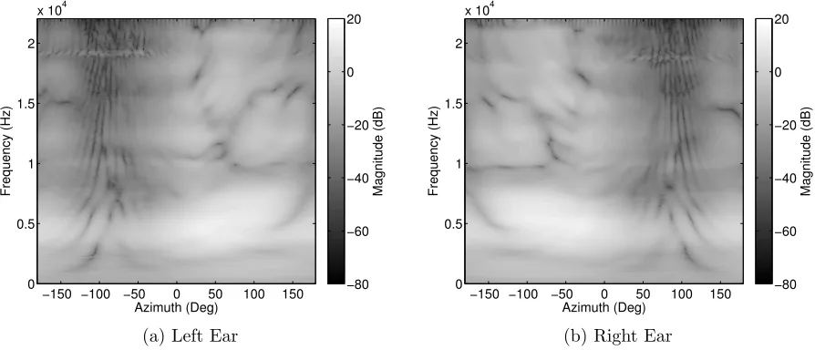
Figure 3.1.4: Measured HRTFs

Figure 3.1.4 shows the magnitude spectra of the measured head related transfer functions for each ear obtained as 20log10of the 2048 point Fourier transform of the measured HRIRs.

The lightest regions between the axes of angle and frequency represent the larger magni-tudes of the measured responses, the largest magnimagni-tudes occur around the ipsilateral source positions between approximately 2kHz and 8kHz for each ear. The darkest regions depict the areas of lowest magnitude, considering the contralateral angle positions of each ear and moving South to North along the frequency axis shows the effects of head shading and how such shading varies with frequency. Lower frequencies at the contralateral source positions exhibit low order diffraction patterns, characterised by the semi-periodic minima that occur as a result of the superposition of the sound waves that split to travel around either side of the head, incurring a significant path difference that results in cancellation of the acoustic pressure. At higher frequencies the magnitude at these contralateral positions is significantly lower due to both increased air absorption, and the increased directivity of high frequency sound (less diffraction).

(46)

of the HRIR measurement set in figures 3.1.2 and 3.1.3, a fundamental means of compression may be achieved through the truncation of the measured impulse responses to include the important region of excitation, including the variable onset delay. The measured impulse responses are of length 2048 samples, however upon simple visual inspection it seems that the latter portion of the responses contains little to no aptitude variation. To ensure that no significant information is lost in truncation, the energy in the impulse response should be considered as a basis for determining the truncation value.

The energy decay curve was defined by Schroeder [1965] as a means of measuring and defining the reverberation time of a space using the impulse response. The energy decay curve (EDC) is defined as the reverse integral of the squared impulse response at timet and describes the total signal energy remaining in the impulse response at that time:

EDC(t)≡

Z ∞

t

h2(t)dt (3.1.1)

In order to select an appropriate truncation length, the EDC of the impulse response corre-sponding to the contralateral source position measured at the left ear is plotted. Logically the contralateral impulse response should have the slowest decay of energy, partially due to its minimal total energy, and partially due to the almost exclusive presence of lower frequency diffracted frequencies at the occluded ear.

0 500 1000 1500 2000 −100

−80 −60 −40 −20 0

Sample No

Energy Decay in (dB)

Ipsilateral Contralateral

(47)

Figure 3.1.5 shows the energy decay curve of the ipsilateral and contralateral impulse re-sponses measured at the left ear, for illustrative purposes both curves have been normalised to the total energy of the ipsilateral HRIR. Considering the values of each curve at the first sample shows that the contralateral HRIR has approximately 20dB less total energy than the ipsilateral, this is of course due to the previously mentioned effects of head shadowing. Both curves converge around -40dB approximately 500 samples into the responses, after which they exhibit a similar decay over the remaining IR length. In the latter region the curves do diverge up to a maximum of ∼5dB, the similarity between the curves in this region suggests that it is likely that this region is dominated by noise in the measured HRIRs. The relatively gentle decay is an artefact of the reverse Schroeder integration technique used to calculate the curves, the HRIRs are reversed and then summed from beginning to end, as such the noise floor in the measurements would yield a steady yet likely shallow gradient in the curve as the cumulative energy in the noise with respect to time increases. The ∼5dB deviation between the curves in the latter 1500 sample region is most likely due to the lower signal to noise ratio of the contralateral HRIR; as less of the total energy in the signal is due to the sound emanating from the source on the other side of the head, more of the total energy in the signal is due to the noise, subsequently the relative contribution of the noise dominated region of the EDC will be greater than that of the ipsilateral counterpart.

The fact that the energy decay curves shown in figure 3.1.5 both seem to exhibit a noise dom-inated response after approximately 500 samples suggests that the HRIRs can be truncated to a 512 sample length with no significant loss of any pertinent binaural cues. Taking the 512 and 2048 point Fourier transforms of the truncated and full length HRIRs respectively was found to yield no discernible truncation effects such as the Gibb’s phenomenon.

3.2 ITD Extraction

(48)

that the key ITD information can be synthesised as required simply by zero padding of the processed minimum phase impulse responses.

This section of the thesis presents a brief comparison of a number of previously identified techniques for the extraction of the ITD applied to the TU Berlin dataset, and leads to the selection and justification of the method that is used in later reconstructions.

−150 −100 −50 0 50 100 150

−8 −6 −4 −2 0 2 4 6 8

x 10−4

Angle (deg)

ITD (Sec)

Spherical Model IACC

(a) IACC

−150 −100 −50 0 50 100 150

−8 −6 −4 −2 0 2 4 6 8

x 10−4

Angle (deg)

ITD (Sec)

Spherical Model IACCe

(b) IACCe

−150 −100 −50 0 50 100 150

−8 −6 −4 −2 0 2 4 6 8

x 10−4

Angle (deg)

ITD (Sec)

Spherical Model Edge Detection

(c) Edge Detection

−150 −100 −50 0 50 100 150 −8 −6 −4 −2 0 2 4 6 8

x 10−4

Angle (deg)

ITD (Sec)

Spherical Model IGD(0Hz)

[image:48.612.84.521.243.646.2]

(d) IGD0Hz

(49)

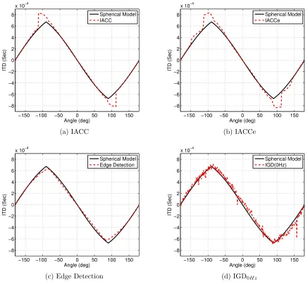
Figure 3.2.1 shows the ITD with respect to angle extracted from the measured Tu Berlin data using each of the four methods. The resulting ITD curve for each method has been plotted against the reference curve of the spherical head model ITD prediction, the spherical head model provides a useful measurement independent reference for the Tu Berlin data as it is known to give a good estimation of ITD in the azimuthal plane, but also because the Tu Berlin data was measured using the KEMAR mannequin and as such should fit well with the approximation of a spherical head.

For the first three methods; the IACC, IACCe, and Edge Detection, the measured impulse responses are first up sampled by a factor of 20, in order to alleviate errors in the ITD time calculation in seconds that is imposed by the measurement sample rate of 44100Hz.

The IACC derived ITD curve shown in figure 3.2.1a was calculated by first computing the cross-correlation function between the left and right ear measurements for each angle using

the xcorr.m function in MATLAB, and then finding the lag value, in samples, for which the

maximum of each function occurs. These sample values are then divided by the sample rate of the original measurement and the up sampling factor to obtain ITD values in terms of seconds.

The ITD curve derived using the IACCe method as shown in 3.2.1b is computed using the same method as the IACC, the only difference is that the cross-correlation of the envelopes of the left and right ear impulse responses is taken rather than of the raw signals. The impulse response envelopes are calculated as the magnitude of the Hilbert analytical signal for each of the left and right signals respectively using the hilbert.m function.

Efficient and compact representations of head related transfer functions