EPSIM An integrated sequential interindustry model for energy planning: evaluating economic, eletrical, environmental and health dimensions of new power plants

Munich Personal RePEc Archive

EPSIM - An integrated sequential

interindustry model for energy planning:

evaluating economic, eletrical,

environmental and health dimensions of

new power plants

Avelino, Andre F. T. and Hewings, Geoffrey J.D. and

Guilhoto, Joaquim José Martins

Universidade de São Paulo, University of Illinois

2011

Online at

https://mpra.ub.uni-muenchen.de/54370/

EPSIM - An Integrated Sequential Interindustry Model for

Energy Planning: evaluating economic, electrical, environmental

and health dimensions of new power plants

Andre F. T. Avelino

, Geoffrey J. D. Hewings

Joaquim J. M. Guilhoto

Abstract

Energy is the input in which modern society depends the most for life standard maintenance besides economic and social activities, however, it is also one of the major sources of greenhouse gases (GHG) emissions, especially the electric sector, due to a world energy matrix concentrated on oil and coal resources. Hereby, impact analysis is essential for policy making focused on sustainable energy systems, once it provides ex ante evaluations for the diverse effects of new projects, being especially important in relation to large infra-structure investments as power plants. In the Brazilian case, although the current electrical matrix is primarily renewable and has low GHG intensity, the required expansion of generation capacity leads to rediscuss power plants’ alternatives and their externalities. Due to the transient and heterogeneous demand of these projects, economic, environmental, energy and social impacts must be assessed dynamically and spatially. This study proposes a social-environmental economic model, based on Regional Sequential Interindustry Model (SIM) integrated with geoprocessing data, in order to identify economic, pollution and public health impacts in state and county levels for energy planning analysis. Integrating I-O framework with electrical and dispersion models, dose-response functions and GIS data, this

model aims to expand policy makers’ scope of analysis and provide an auxiliary tool to

assess energy planning scenarios in Brazil. Moreover, a case study for wind power plants in Brazil is performed to illustrate its usage.

Keywords: Energy Planning; Input-Output; Sequential Interindustry Model; Energy Economics

1. Introduction

The electrical sector is responsible for a considerable amount of greenhouse gases emissions worldwide, but also the one in which modern society depends the most for maintenance of quality of life as well as the functioning of economic and social activities. The Kyoto Protocol and IPCC (Intergovernmental Panel on Climate Change) reports on

1 _{School of Economics, Business Administration and Accountancy – FEA/USP, Rua Luciano Gualberto, 908}

São Paulo, SP – Zip Code: 05508-010. E-mail: [email protected]. Phone: (11) 9406-7425

2 _{Regional Economics Application Laboratory (R.E.A.L) – University of Illinois, UIUC, 607 S. Matthews}

Street, Urbana, IL – Zip Code: 61801-3671. E-mail: [email protected]. Phone: +1-217-333-4740

3 _{School of Economics, Business Administration and Accountancy – FEA/USP, Rua Luciano Gualberto, 908}

climate change issues identify sustainable development and rational resources use as key points to future. Thus, energy planning should consider not only economic impacts, but also environmental and social effects during the entire investment life cycle and idiosyncrasies of the chosen location.

Brazilian energy matrix is one of the least polluting in the world, especially due to its domestic electricity supply, which has low pollutant emission indexes since it is concentrated in renewable energy sources (90.6%). Nevertheless, the generation portfolio is not too diversified with predominant supply of hydropower plants (76.9%) and low shares of other

“clean” sources such as biomass (5.4%), nuclear (2.5%) and wind (0.2%), which increase energy security issues (MME, 2010).

Since 2003 an electricity consumption rebound has raised per capita growth rates to 5% annually in Brazil (TOLMASQUIM, 2005). During all this phase, income elasticity measures for electricity consumption were superior to the unit, which has reflected in a consumption expansion higher than annual GDP growth and an increasing demand for generation infra-structure. In order to comply with this new scenario, several projects have been undertaken in the last years, particularly new wind, gas-fired and thermonuclear plants (ANÁLISE, 2010).

Considering the fact that 22% of all greenhouse gas emissions come from energy use in the Brazilian case (MCT, 2009), which includes the electricity sector, it becomes essential to discuss externalities of the energy sources chosen in electricity generation expansion. Variables such as amount of pollution, power plant location and population density affects diversely public health and are important to be accounted for during energy planning.

Several epidemiological studies have confirmed that even short term exposure to non-recommended levels of pollutants may lead to increases in mortality rates and development of different morbidities (POPE, 2000). Nevertheless, pollutants concentration varies across regions due to the location of emission sources, microclimate dynamic, topography, weather and other factors, confirming the importance of a spatial analysis. Moreover, it is important to notice that pollutants emissions and climate changes have a reflexive effect both on the electricity system – affecting the own efficiency of certain power plants at low air quality levels – and in the local and national economy – due to demand shifts, lost working days and increase use of the health care sector.

In sum, recent scenario leads to new discussions about electricity generation portfolios that must be expanded and diversified under the premises of environmental sustainability. Due to these new parameters, different power plants must be assessed not only financially, but also socio-environmentally, considering regional idiosyncrasies, as this study intends. The proposed model allows assessing externalities in different regions and

advantages/disadvantages of different sites for a power plant’s project. It is composed by a

set of Regional Input-Output matrixes for Brazil and three other modules integrated computationally: Environmental Module, Energy Module and Health Module.

In the next section we describe the proposed model, discussing each module separately, followed by the dataset used in section three. The study case for Osorio Wind Farm is presented and analyzed in section four and conclusions follow.

2.1. Overview

Impact analysis is an essential feature for policy making providing ex ante evaluations for the effects of new projects and it is especially important in relation to large infra-structure

investments. In the case of energy planning, ex ante evaluations are performed quite before

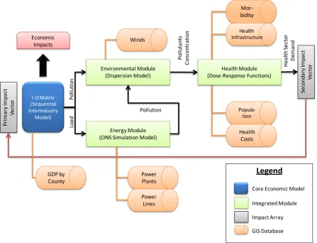
the beginning of a project (construction of power plants, substations and transmission lines) and involve assessing several options, construction sites and their induced regional impacts. One must notice that besides cost differences, also economic multipliers, emissions and public health impacts differ spatially and a balance of positive and negative externalities shall be considered in energy expansion. Moreover, impact analysis allows addressing benefits and issues different actors (decision-makers, enterprises, organizations and population) will perceive across regions.

Figure 1 – General vision of the model

The primary characteristic of large construction projects is their transient nature (ROMANOFF; LEVINE, 1980), i.e., economic impulses (demands) are heterogeneous through time. Their construction, in particular power plants, extends throughout several years before completion. Hence, these projects should not be addressed by static models, which compromise the accuracy of the analysis. The comparison of an equilibrium state before

Legend P ri m a ry Im p a c t V ec to

r I-O Matrix (Sequential Interindustry

Model)

Energy Module (ONS Simulation Model)

S e c o n d a ry Im p a c t V e c to r Economic Impacts P o ll u ti o n L o a d Pollution P o ll u ta n ts C o n c en tr a ti o n He a lt h S ec to r D em a n d Power Plants GDP by County Power Lines Winds Mor-bidity Health Infrastructure Popula-tion Health Costs Health Module (Dose-Response Functions) Environmental Module (Dispersion Model)

Core Economic Model

Integrated Module

Impact Array

construction and the new equilibrium after construction neglects the existing dynamic in-between theses two time periods. Construction is a complex sequential operation which demands different industrial and non-industrial inputs in subsequent phases. As each project has a unique cost, location and technology, distinct evaluations must be performed for each project individually and impact analysis is not transferable to other projects.

The proposed model is divided into four interconnected components – (1) Core

Economic Model; (2) Environmental Module; (3) Energy Module; and (4) Health Module –

with a feedback system in the end of the process to iterate the algorithm. The model is computationally built and it allows assessing benefits and downsides of different construction sites for a power plant’s project and their regional externalities (Figure 1).

Using a regional Sequential Interindustry Model (SIM), direct and indirect economic impacts of the construction phase of the power plant are estimated for each region. The advantage of using a SIM is being able to analyze how irregular demand flows in different stages of construction dynamically impact the economy over several time periods. Then, once pollution coefficients are determined for each industry type, it is possible to estimate total pollution generated by the economy and the location of these emissions. Total pollution has, thus, two dimensions: physical units of the pollutant and source location. These variables are inputs to the Environmental Module which assesses the dispersion of pollutants, and forecasts their concentration in each location.

The required industrial output for the construction also raises the demand for electricity, which must be supplied with extra generation. The Energy Module emulates the

grid operator’s (ONS) wheeling system and is applied to determine which power plants will be dispatched and consequent emissions by location. These outputs are also inputs for the Environmental Module. Finally, pollutants concentrations by location are applied in the Health Module that estimates the demand for health services/products in different regions. This demand is a new shock vector for the Input-Output matrixes that enters the process in an iterative fashion.

Geoprocessing information is used in several databases, providing information about population, wind speed, public health services, etc. for each location. A spatial vision of the entire process is achieved, allowing analysis of results in an aggregated way (economic, environmental and public health total impact) or disaggregated by region, thereby revealing more sensitive locations to pollution problems and/or economic benefits.

2.2. Economic Module

Input-Output (I-O) models allow a detail vision of both macroeconomic and microeconomic impact of policy effects in a certain region, through the analysis of industrial interdependency within an economy. In the economy, the production of a good or service has two consumption destinations: either be directly consumed by final demand or used as input

in the production of another good/service (intermediary consumption). Denoting by Xi sector

i total production, z the intermediary consumption of its production by n sectors of the

economy (including the consumption of the own industry) and Yi final demand of sector i’s

It is important to state an intrinsic hypothesis to this I-O Model: interindustrial flows from i to j, for example, depends entirely on sector j’s total production in a certain time horizon. The technical coefficient (aij) is the relation between the share of sector j’s

production used by sector i (zij) and sector j’s total production (Xj). It is supposed constant

according to the premise of constant returns of scale (MILLER; BLAIR, 2009).

Fixed technical coefficients imply a methodology limitation once the own economy dynamics causes coefficient variations over time and consequently, analysis and inferences of the models are valid only to a short term horizon (LABANDEIRA; LABEAGA, 2002). Replacing (2) in (1), rearranging in matrix form and solving the equations to determinate total output required to final demand (Y):

(I – A)-1 is Leontief Inverse, which indicates all requirements for the economy’s

production, direct (from final demand) and indirect (from intermediary demand). It reflects how final demand propagates inside the entire economy (MILLER; BLAIR, 2009).

The Sequential Interindustrial Model (SIM) is built on the static I-O model with the insertion of a chronology in industrial processes. SIM is based on time-phased production, i.e., production process occurs sequentially in time, differently from the static I-O model which assumes that production occurs simultaneously during a single time-step. With this flexibility, one may represent different stages of manufacturing and transportation to final use, enabling to assess transient phenomena as the construction of power plants (ROMANOFF; LEVINE, 1981).

Two hypotheses must be made for the time interval k: (1) k is equal for all industries and constant through time; and (2) all industry intervals are synchronized (ROMANOFF; LEVINE, 1981). Without these assumptions, there would not be feasible to formalize the model with difference equations and approach solutions which could be assess using traditional I-O framework.

Recalling the fundamental relation expressed in Eq. 1 and assuming that time is partitioned into discrete industry intervals, during the kth interval the I-O model can be rewritten as:

Eq. 1

Eq. 2

Eq. 3

Next step would be determining the coefficient matrix A for the economy. Nevertheless, as two production process with distinguish dynamics exist, responsive and anticipatory industries will differ in relation to time steps required. In the responsive model, the intermediate yield is expressed as:

Meaning that intermediate yield at interval k is linked to total supply at interval k-1. On the contrary, in the anticipatory model, intermediate yield at interval k is supposed to be linked to total supply at interval k+1, resulting in:

The responsive model is derived by replacing Eq. 5 into Eq. 4 and the anticipatory model by replacing Eq. 6 into Eq. 4. Finally, using the double-sided Z transform one derives de pure responsive model and the pure anticipatory model, respectively:

∑

∑

However, as the economic structure is composed of both anticipatory and responsive industries, one needs to define a mixed model which comprises the two production processes. This system may be formalized as:

Hence, the solution takes the form:

∑

Where Gr(A1,A2) is a matrix function which has all path gains by the industries until

time period k. This single region model may also be translated into an interregional model if one considers the matrixes in Eq. 9 as compositions of regional matrixes. Hence, for a two regions (L and M) example:

[ ] [ ] [

] [

] [

] [ ]

Eq. 5

Eq. 6

Eq. 7

Eq.8

Eq. 9

Eq. 10

The only difference between pure systems and the mixed one is the production chronology. The production output of the former models is equal to the mixed production model, and also equal to that of the static I-O model.

In order to analyze the interface within industrial dynamic, pollutants emissions and additional electricity load, two extensions are required. Considering only two regions L and M, firstly, a pollution intensity (p) vector, which measures the amount of pollution emitted by industries in each region (tons of pollutant / R$ Million), is determined for each industry:

Where TPL is a vector comprising total emissions discharged in one year for each industry in region L. One must note that the electricity sector does not have a coefficient, once it will be estimated separately, using the Energy Module, avoiding double counting. Secondly, it is defined an auxiliary vector for energy intensity (e) that determines electrical consumption required (MWh) to produce R$ 1 million of a certain sector i at region L:

Where CTEL _{is an}

nx1 vector with total electrical consumption in one year for each industry region L. This definition, however, differs from the engineering definition of energy intensity. Intensity, in engineering, is equal to total energy requirement divided by added value in the product; in this paper, energy intensity is measured by total energy requirement divided by total production value, not just added value.

Aggregating the vectors p and e and considering the resumed form for the

interregional model, analysis is done in two steps: first, we calculate total production (Ẋ),

direct and indirect impacts, from the power plant construction demand (Ẏ). These values are

converted into emissions in order to determine total pollutants released during implantation ( _̇ ). The _̇ vector contains pollution released by each industry in each region. It is the output of the economic model to the Environmental Module (pollution by location). Second, we estimate the electricity load for the construction ( _̇ ) by postmultiplying the diagonalized total production (Ẋ) by the energy intensity vector (e). This vector contains electricity requirements by industry in each region and is the output of the economic model to the Energy Module (electricity by location). These vectors also have a time dimension from the SIM model.

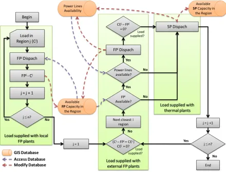
2.3. Energy Module

The Energy Module simulates the dynamic of the wheeling of the grid, which must

maintain a static and a dynamic equilibria in order to keep the system’s integrity. The basic

operational idea for the grid administration is to minimize the energy price to consumers, subject to the transmission lines constrains. The concept is that inflexible power plants (hydropower, nuclear, wind and some thermal) are always connected to the grid and, thus, if there is an extra load in the system, they are preferred to increase generation to attend this demand.

Eq. 12

In order to simulate the wheeling performed by ONS, NOWSS program was developed. The National Operator Wheeling System Simulation (NOWSS) is a simplified version of the network procedures and it is not intended to precisely estimate the energy flows and power plants but to show trends in the grid. The NOWSS is used to forecast a monthly dispatch due to extra loads in the grid and not to simulate daily operations. The

program’s inputs are monthly extra loads by state and the output total generation by plant. Three important assumptions are made in this model due to its simplicity: (1) only interstate lines are considered (136 lines) and the transmission capacity is limited by the characteristics of the power lines; (2) it is assumed that each state has only one substation and all power plants in this state are connected without distance costs to it. This substation is responsible for receiving and sending electricity to other states, distribute it to consumers and has no capacity limitations (the power lines create this limit); (3) power plants are classified in first priority (FP), facilities always connected to the grid composing the baseload, or second priority (SP), complementary generation.

Figure 2 – Simplified overview of NOWSS algorithm for n regions

The program minimizes costs between supply and demand, accounting for transmission distance and plants’ priorities. Substation and lines form a graph with 27 vertices and 136 edges. The edges are oriented (energy flow can only follow one direction in the same line) and one or more edges can connect two vertices. The weight of each edge

Load supplied with thermal plants

Load supplied with external FP plants Load supplied with local

FP plants Load in Region j (Cj₎

FPj_Dispach

j = 1

Load supplied? (Cj_–FPj_{= CE}j ₎

CEj _{= 0?} j ≤n?

Next closest i region j = j + 1

Load supplied? CEj_–FPi

= 0? SP Dispach

j ≤n? j = j +1

End No Yes No Begin Available FPCapacity in

the Region

FPi Available?

Available SPCapacity in

the Region Power Lines

Availability

FPj_{- C}j

Power lines available? FPi_Dispach

depends on the line capacity and an edge cannot be used anymore if its transmission limit is reached.

Before being able to forecast the dynamic of an extra load in the SIN, the NOWSS calculates the steady-state of the system, i.e., which power plants and power lines are used to balance the grid in a regular monthly operation. This provides information about available generation capacity and paths for electricity transmission for the second step. Once the system reaches a steady-state and information about available power lines and power plants are estimated, the program can perform the grid wheeling to allocate extra loads subject to these restrictions.

The algorithm initially checks if there is available FP plants in the state or nearby regions to supply the extra load. If SP plants are required, it searches the graph for the least expensive thermal plant to dispatch, which depends on the cost of generation and transmission distance (Figure 2). The algorithm is similar to Dijkstra’s for finding the shortest paths between a source and every other vertex, however not only edges have different lengths, but vertices have different weights. After a new steady-state is reached, pollution from dispatched thermal plants is estimated and sent to the Environmental Module (total emission, location and time period).

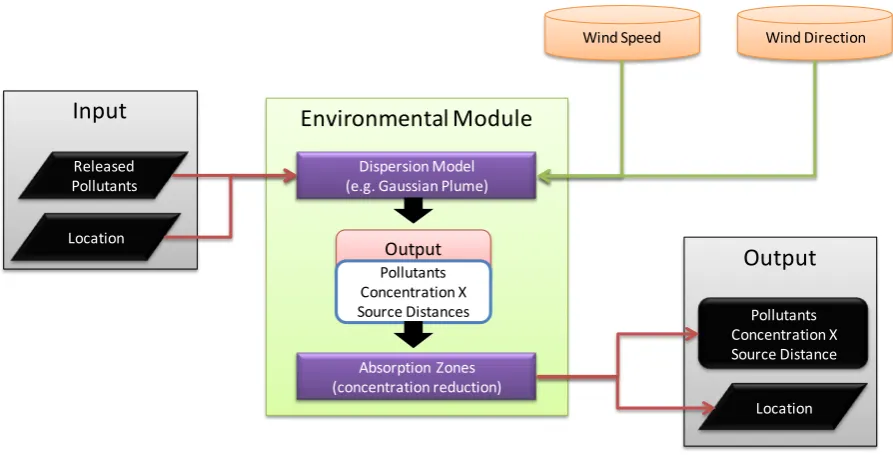
2.4. Environmental Module

Both Economic and Energy modules send a dataset to the Environmental Module containing quantity of pollutants released to the atmosphere (and type) and the location of the source by time period (Figure 3). Using GIS data for meteorological conditions, a Gaussian Plume Model (GPM) is applied for each region to determine the total concentration of pollutants at different distances from the source, considering the effect of one region in another.

Figure 3 – Environmental Module

Environmental Module Input

Output

Released Pollutants

Wind Direction

Dispersion Model (e.g. Gaussian Plume)

Location

Absorption Zones (concentration reduction)

Pollutants Concentration X Source Distances

Output

Pollutants Concentration X Source Distance

Wind Speed

Pollutants are carried by wind and diluted by atmospheric turbulence until final deposition in the ground. Some compounds may react in the atmosphere and form secondary pollutants like H2SO4 and O3. As in this study only primary pollutants are assessed and they

are chemically stable close to the emission source, a simple Gaussian Plume Model (GPM) can be used to predict pollutants concentration.

GPM assumes that continuously released pollutants are carried in a straight line by the wind and mix with the air both horizontally and vertically resulting in pollutant concentration with a normal (Gaussian) spatial distribution (EUROPEAN COMMISSION, 2005).

We use a simple GPM without extensions to account for chemical reactions, considering a homogeneous emission rate throughout the time period and concentration at ground level only. It is formalized as:

{ (

) (

)} {

}

Where c(x,y,z) is the atmospheric concentration at any point x meters downwind of

the source, y laterally from the centerline of the plume and z meters above ground level; Q:

emission rate; u: wind speed; h: stack height; σy: cross wind standard deviation (measure of plume width); and σZ: vertical standard deviation. For the plume to dislocate in the air in a straight line at constant speed, two other assumptions are made for GPM: (1) flat terrain and (2) constant meteorological local conditions. Moreover, vertical wind shear is not considered. Through this model one may assess the concentration of pollutants as far as 100 km from the emission source (SALBY, 1996). The model will be used to estimate the concentration due to industrial emissions and power plant emissions. The accuracy of the analysis, however, will vary depending on the source: once exact location of industries is not available, it is assumed that for a certain county industrial mix is homogeneously distributed throughout the region; for power plants, location is precise (latitude/longitude).

Considering wind speed and bearing in different seasons, the final output of the model is concentration of pollutants by distance from source at several time periods. This data is used in the Health Module for public health impact evaluation.

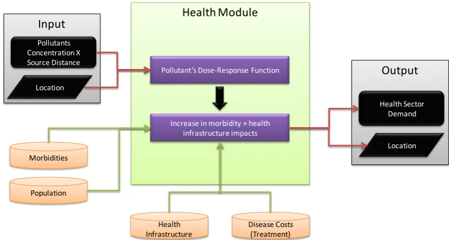
2.5. Health Module

The Health Module receives concentration data, with location and time period, for each pollutant considered in the Environmental Module (Figure 4). Adding it to preexisting pollution on site at time period k, total pollutants concentration (pck) can be estimated by

region. Then, deleterious effects are forecasted through dose-response functions (DRF) which calculate the increased probability of pollution-related diseases (morbidity rate – impacts on mortality rates are not considered) and estimate the health sector demand caused by this non-recommended exposure. DRFs relate the concentration of pollutants an agent is been exposed to the physical impact on this receptor. We consider that the DRFs do not have any threshold

point, as has been discussed by Pope (2000). The impacts of NO2 and SO2 are assumed to

increase indirectly from the particulate nature of nitrate and sulfate aerosols, and CO2 impact

is measured by CO effects (which derives from an inefficient combustion of CO2).

In order to transform public health effects into demand for health care services, the average cost per patient admitted in public hospitals is considered for each type of disease (costdisease), besides the last hospital admission rate by region (admisk-1). The final

monetization of impacts is accomplished by estimating the number of excess diseases due to the pollution (admisk-1*DRF()) and multiplying it by the treatment cost for each disease.

Hence, for region L, the health sector demand at time k (hkL) depends on the current number

of hospitalizations, the increase in morbidity cases and the local treatment cost:

It is important to notice that although the number of cases increases in a certain region, the effective health demand may not occur in this region due to a lack of available health care services. Hence, we consider that population can migrate to nearby regions seeking for treatment. Finally, total health care demand is estimated and transformed into a new shock vector which iterates the model.

Figure 4 – Health Module

3. Databases and Software

The national I-O matrix for Brazil was derived according to the methodology presented in Guilhoto and Sesso Filho (2005a), while the estimation of the interregional I-O system was made following the methodology presented in Guilhoto and Sesso Filho (2005b). The 2004 matrix is divided into 12 sectors and 27 regions (26 states and Brasília). This level

Health Module Input

Pollutants Concentration X Source Distance

Location

Increase in morbidity + health infrastructure impacts

Output

Health Sector Demand

Location

Pollutant’s Dose-Response Function

Population Morbidities

Health Infrastructure

of aggregation was necessary to match industries with emission data from MCT (2009). In further works more disaggregated data shall be used.

In order to create a mixed SIM, these sectors were classified into responsive and anticipatory production mode. As highlighted by Romanoff and Levine (1986), anticipatory mode is usual in sectors as agriculture, mining and manufacturing industries, in which production typically anticipates orders with readymade standard products. Responsive mode, in the other hand, is a characteristic of construction, ordinance, services and industries in contract research and development work, once they usually respond to custom orders,

according to costumers’ specifications. Sectors and their classification can be seen in Appendix 1. Moreover, the time step k is considered monthly intervals.

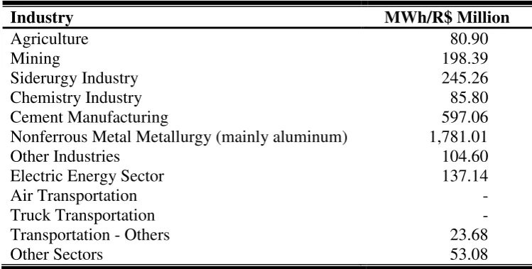
Database for the Energy Module is based on ONS (2010) information on power plants and transmission lines. For the first step of the program, data regarding the usual load for each state is required. In order to be consistent with the economic database, the share of consumption by state for 2002 is used to estimate 2004 electricity consumption (ANEEL, 2005). As NOWSS estimate the monthly dispatch dynamic, seasonal effects on capacity factors must be accounted for, especially for wind and hydropower plants. Data from ONS (2010) for 2004 is used to forecast the average capacity factor by plant in each month. Moreover, average generation was estimated for each plant from weekly reports also from ONS. The latter, however, is based on 2007 reports due to unavailable reports for 2004.

For the cost of SP plants, the NODAL Program V3.4 (ANEEL, 2010) was loaded with parameters for 2007/2008 period and RAP = R$ 6,985,975,595.08. These variables are used to weight each vertex in the graph for the path optimization. For the extra load wheeling, energy coefficients by industry type were estimated with ECEN (2010) data regarding 2004 consumption. In that year total industry and commerce consumed 310,017 GWh and households 86,695 GWh. Coefficients can be seen in Table 1 below.

Table 1 – Electricity consumption coefficients by industry

Industry MWh/R$ Million

Agriculture 80.90

Mining 198.39

Siderurgy Industry 245.26

Chemistry Industry 85.80

Cement Manufacturing 597.06

Nonferrous Metal Metallurgy (mainly aluminum) 1,781.01

Other Industries 104.60

Electric Energy Sector 137.14

Air Transportation -

Truck Transportation -

Transportation - Others 23.68

Other Sectors 53.08

Source: Based on ECEN (2010).

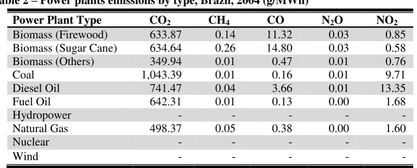
density). This level of details allows a more accurate analysis of pollutants concentration and public health effects. Emission coefficients for each type of power plant regarding different pollutants were estimated based on ECEN (2010) with data from the National Energy Balance for 2004 and results can be seen in Table 2. In our model, however, only CO and NO2 levels will be assessed.

For industrial emissions, there is not a database for industries’ locations, fact that limits the scope of the analysis. The proxy used is: given the economic structure of a state (from the I-O matrix), each county is allocated with a share proportional to its industrial GDP, and industries are homogenously distributed throughout this region. Data from

industrial GDP is taken from IBGE (2010). CO2 emissions are estimated based on individual

coefficients for each industry type, based on MCT (2009) for 2004 pollution. The only sector

without emissions is “Electric Energy Sector” to avoid double counting with the Energy

Module. In order to obtain CO and NO2 levels, based on data for 2004 from ECEN (2010),

two additional conversion coefficients were set: 1 ton CO2 = 0.0128 ton CO; and 1 ton CO2 =

0.0028 ton NO2.

Table 2 – Power plants emissions by type, Brazil, 2004 (g/MWh)

Power Plant Type CO2 CH4 CO N2O NO2

Biomass (Firewood) 633.87 0.14 11.32 0.03 0.85

Biomass (Sugar Cane) 634.64 0.26 14.80 0.03 0.58

Biomass (Others) 349.94 0.01 0.47 0.01 0.76

Coal 1,043.39 0.01 0.16 0.01 9.71

Diesel Oil 741.47 0.04 3.66 0.01 13.35

Fuel Oil 642.31 0.01 0.13 0.00 1.68

Hydropower - - - - -

Natural Gas 498.37 0.05 0.38 0.00 1.60

Nuclear - - - - -

Wind - - - - -

Source: Based on ECEN (2010).

Moreover, for simplification, all terrain in Brazil is considered flat to avoid the need for further appendices to the GPM. GIS information regarding wind speed, bearing and latitude/longitude at county level is available in CEPEL (SWEARA, 2010) for 10km x 10km cells. This database refers to simulations generated in MesoMap for 360 days from a period of 15 years of data with each month and season being considered in a representative way.

The most comprehensive available emission data for Brazil covers CO2, CH4, N2O,

HFC-23, HFC-134, CF4, C2F6 and CF6 (MCT, 2009). But detailed disaggregation is given to

the first three pollutants only. Therefore, carbon dioxide, methane and nitrous oxide can be analyzed. Methane is not a toxic gas, hence, its health effects will be neglected. Carbon dioxide will be evaluated through CO impacts and nitrous oxide will be measured as nitrogen oxide. The DRFs used in this work are based on Gouveia et al (2006) study and are summarized in Table 3. In their study the sample is divided into children and elderly but we use a conservative number to represent an average adult response.

several cities there is access to private health care services, the majority of the Brazilian population (90%) still relies on public health services. Moreover, as high pollutant industries and power plants are usually located in peripheral urban areas, low income population is more susceptible to suffer from pollution effects. Hence, data from SUS is a good approach to the real health costs incurred. DATASUS (2010) has a large database with the number of hospital admissions by disease, total treatment cost, hospitalization period, mortality rate, etc., by Federal, state and county levels for the SUS system. This database will be used to assess public health impacts.

Table 3 – Increase in morbidity due to 10 μg/m3 _{raise in NO}

2 and CO concentrations

NO2 CO

Asthma 2.3% 5.4%

Pneumonia 0.8% 3.9%

Other Respiratory Diseases 1.2% 2.4%

Cardiovascular Diseases 1.0% 1.6%

Source: Adapted from Gouveia et al, 2006.

The model proposed was programmed in Pascal language using Borland Delphi 5 environment and the final software is entitled EPSIM (Energy Planning Sequential Interindustry Model). The program was built in five different units (four modules and an iteration routine) and operates in both state and county levels (27 states and 5560 counties).

In this initial version (implementation 1.5), it was designed to evaluate impacts for construction phase only (further works will address operation and decommission). The economic and energy modules operate in state level while the other modules operate in county level. The user must input an initial shock vector (construction demand) with temporal dimension in order to initiate the program.

4. Case Study

4.1. Scenario

This case study is based on Osorio Wind Farm located in Rio Grande do Sul, Brazil. Data for this wind power plant was based on Osorio Wind Park that reached full operation in 2007 with 150 MW installed. For construction phase, expenses structure was estimated with information on total construction costs (R$ 670 million) and materials from Ventos do Sul Company (2007). They were allocated according to an international expenses average for wind farms (WINROCK INTERNATIONAL, 2004) (Appendix 2).

In order to illustrate the model usage, a comparison is made between three Brazilian states suitable for wind farms investments: Rio Grande do Sul (RS), Ceará (CE) and Rio

Grande do Norte (RN) –by convention, these states are denoted “primary states”. We assume

4.2. Results and Discussion

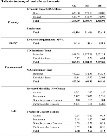
A summary of results for economic, energy, environmental and health impacts is shown in Table 4 below. Overall, results confirm the importance of assessing impacts in both spatial and temporal dimensions, once regional idiosyncrasies imply different effects for each scenario.

Table 4 – Summary of results for each scenario

CE RN RS

Economy

Economic Impact (R$ Millions)

Direct 670.00 670.00 670.00

Indirect 588.39 639.74 648.98

Total 1,258.39 1,309.74 1,318.98

Employment

Total 41,494 51,416 27,619

Energy

Electricity Requirements (MWh)

Total 142.4 149.4 153.6

Environmental

CO Emissions (Tons)

Industries 1,861.58 1,977.28 2,022.24

Electricity Sector 5.17 7.28 6.84

Total 1,866.75 1,984.56 2,029.08

NO2 Emissions (Tons)

Industries 407.22 432.53 442.36

Electricity Sector 19.84 27.77 25.94

Total 427.06 460.30 468.30

Health

Increased Morbidity (Nr of cases)

Asthma 1,042 395 450

Pneumonia 2,997 2,072 2,331

Other Respiratory Diseases 370 216 284

Cardiovascular Diseases 2,095 1,361 1,785

Treatment Cost (R$ Millions)

Asthma 0.54 0.22 0.25

Pneumonia 2.48 1.77 2.03

Other Respiratory Diseases 0.39 0.21 0.28

Cardiovascular Diseases 0.67 0.44 0.56

Total 4.08 2.64 3.12

Total economic impact (direct and indirect) due to the construction was very similar in RS and RN (R$ 1,319 million and R$ 1,310 million respectively), once overall regional output multipliers in these states are close. However, as in RS intraregional and interregional multipliers with SP and MG are larger than in RN, total economic impact was slightly higher in the former. In the case of CE (R$ 1,259 million), lower output multipliers imply reduced effects in comparison with the other scenarios.

Regarding economic spillovers, one may notice that effects for RS scenario are concentrated in the South and Southeast regions, while for CE and RN scenarios, impacts are also observed in the Northeast region but major economic leakages are still located in the Southeast region (Figure 5 and Figure 6). This reflects the industrial structure of each region, once South and Southeast states concentrate around 78% of the 2004 industrial GDP (IBGE, 2010) and supply the Northeast region.

Figure 5 – Total economic impact by state (RS, CE and RN scenarios)

Moreover, results also corroborate with the fact that states of SP, MG and RJ are the most important suppliers to the country, serving as major outputs hubs, due to their industrial and service structure, which represents 53.7% of the national GDP (IBGE, 2010), and strong interregional links with all other states.

due to a labor intensive economic structure, total employment is much higher than in RS case, which impacts mainly capital intensive states. Moreover, most jobs are created during the construction interval and “Agriculture”, “Siderurgy Industry”, “Other Industries” and “Other Sectors” concentrate employment generation in all three scenarios (Appendix 4).

Obs.: The height of the bars represents the share of impact in the state in relation to total economic impact minus effects on primary state (CE, RN or RS).

Figure 6 – Scope of economic spillovers for each scenario

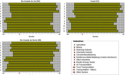
In relation to industrial activation through time, in all scenarios three sectors were demanded before all others: industries not directly related to civil construction, electricity

companies and services (“Other Sectors” mainly), once the construction demand in months zero and one is strictly related to engineering consulting services and expenses prior to construction (Figure 7). On subsequent time periods, “Mining”, “Siderurgy Industry”,

“Chemistry Industry” and “Cement Manufacturing” are continuously demanded until the end

of the construction stimulus. The wider activation time of these sectors is due to the anticipatory production mode assumed. One may also observe a propagation effect beyond the initial 18 months of construction as a result of economic inertia.

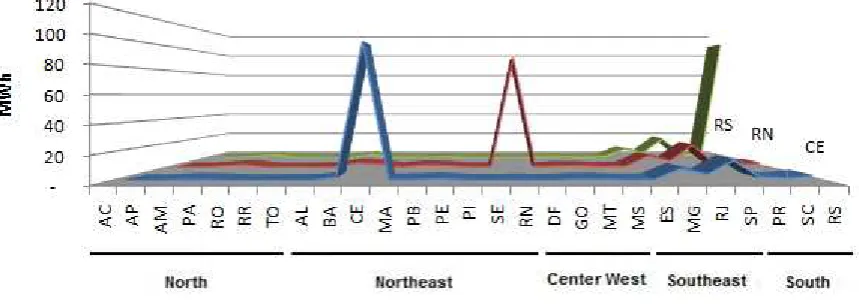
Electricity consumption due exclusively to the construction of the power plant was estimated in 153.6 MWh for RS scenario, 149.4 MWh for RN scenario, 142.4 MWh for CE scenario. Energy requirements pattern is directly related to industrial activation due to economic impacts in each state, as can be noticed by comparing Figures 5 and 8. These electricity requirements are compatible with ONS database, representing less than 1% of total electricity consumption in 2004.

Figure 8 – Energy requirements by state

Total CO and NO2 emissions can be seen in Table 4 and are also related to total

economic impact and energy requirements. Interesting to notice that although part of the emissions are concentrated in the primary state it is also spread to other regions, particularly Southeast states. For CE and RN scenarios, this external negative externality has a particular pattern creating some effects in neighbor states but most of it is concentrated in the Southeast region, causing high pollutants concentrations in SP, MG and RJ (Figure 9). RS emissions also exhibit this effect, however, RS internalizes more industrial emissions (74.8% of CO emissions) and spreads more negative externalities to neighbor states than distance ones (Appendix 5, 6 and 7). NO2 emissions have similar distribution patterns.

Regional idiosyncrasies also influence health impacts in each scenario. Despite the fact that economic impacts and total emissions are higher in RN and RS scenarios than in

CE’s, increase in morbidity and total health costs are larger in the former due to the spatial

Northeast Region. As local CO emissions account for 68% of total emissions, most of the increase in hospital admissions occur in CE and therefore incurs higher treatment costs.

Figure 9 – Total CO concentration by state

Secondly, as can be notice in Appendix 5, 6 and 7, CE and RN have large emission scopes which comprise states in the Northeast, Southeast and South regions. However, in relation to RN, CE creates high pollutants concentration in PE, MA and PI – states with

elevated morbidity rates and treatment costs in the Northeast –, while RN affects

predominantly other Northeastern states. On the contrary, in relation to RS, CE’s higher

morbidity rate is due to a much wider spread in emissions than the former, as highlighted before, and larger concentrations in MG, which has the second highest morbidity rates among all other states.

health costs in period 7 and another in period 14, while CE concentrates expenses during periods 4-7 and exhibit a peak in period 15 and RN follows a similar pattern but with reduced costs (Figure 10).

Figure 10 – Health care demand through time

rates have a significant impact on diseases’ profiles. Due to major health impacts concentrated in the primary states, environmental conditions such as climate, population density and pre-existing pollution lead to an important distinct profile, especially for pneumonia, between northeastern states (CE and RN) and southern states (RS). Therefore, specific health treatments are demanded distinctly in time and in each scenario.

Figure 11 – Increase in hospital admissions by disease in different time periods

5. Conclusions

As pollution is spatially dynamic, i.e. it is emitted at the source but its impacts extend to the length of dispersion it produces, to proper evaluate its externalities, models coupled with spatial components shall be used. In this study, a hybrid top-down/bottom-up model is proposed, coupling a regional economic model with GIS data and electric-social-environmental specifications. For each power plant site, it estimates total economic impacts, effects on the wheeling dynamic of the electric grid and public health impacts due to pollutants dispersion. Through this model, several locations for the construction of a new power plant can be compared regarding positive/negative externalities in the micro-region (state level) and macro-region (country level).

environmental and public health total impact) or disaggregated by region, determining more sensitive locations to pollution problems and/or economic benefits.

The importance of temporal and spatial dimensions in impact analysis could be evidenced in the case study performed for Osorio Wind farm. Although larger economic impacts and pollution were estimated for RS scenario, economic spillovers and emissions were less spread than other construction sites. On the contrary, although CE scenario presented smaller total economic output, it had a larger capacity of jobs creation but a wider spatial scope of negative externalities which translated into higher public health impacts. Regional idiosyncrasies regarding local economic structure, interregional multipliers, emission coefficients and health care infrastructure were essential to perform this more accurate assessment than traditional I-O models. EPSIM software was able to proper address the transient demand from electrical investments and to provide economic, environmental and public health effects in spatial and temporal dimensions for comparisons between different scenarios.

Nevertheless, some limitations in the proposed model must be highlighted: as discussed above, I-O framework is not suitable for long-run forecasts once the economy’ structure changes through time. Thus, considering using a computable general equilibrium (CGE) model is an alternative to better assess economic impacts; the simple GPM presented can be enhanced by adding extensions for airborne chemical reactions; and better databases regarding industrial location, morbidity rates and health care infrastructure in county level shall increase estimations’ accuracy.

In sum, planners can benefit from this model exploring the impacts of diverse energy sources and locations, assessing economic, environmental and social aspects of each alternative. Electricity will still remain as an essential input in the future as well as its environmental concerns. Sustainability is a challenge to be addressed today for a long-term benefit. The more tools society can rely on, better decisions can be made and a cleaner future planned.

6. Acknowledgments

This work was partially developed under CAPES/FIPSE Exchange Program “Global

Talent Development for Sustainable Agricultural & Environment Sciences Fields” with

financial support of CAPES.

7. References

ANÁLISE. Análise Energia: Anuário 2010. São Paulo: Ibep, 2010.

ANEEL. Atlas de Energia Elétrica. Second Edition. Brasília: ANEEL, 2005.

ANEEL. BIG – Banco de Informação de Geração. 2010. Available in: <http://www.aneel.

gov.br/15.htm>. Access in May 28, 2010.

ECEN. Balanço de Carbono, Energia Equivalente e Final: Brasil 1970-2006. Software.

Brasília: MCT, 2010.

EUROPEAN COMMISSION. ExternE – Externalities of Energy: Methodology 2005

DATASUS. Banco de Dados do Sistema Único de Saúde. 2010. Available in: <http://www.datasus.gov.br/>. Access in Aug. 10, 2010.

GOUVEIA, N. et al. Hospitalizações por causas respiratórias e cardiovasculares associadas à

contaminação atmosférica no Município de São Paulo, Brasil. Cadernos de Saúde

Pública, v.22, n.12, pp.2669-2677, 2006.

GUILHOTO, J.; SESSO FILHO, U. Estimação da Matriz Insumo-Produto a partir de Dados

Preliminares das Contas Nacionais. Economia Aplicada, Ribeirão Preto, v.9, n.1,

April-June, 2005a.

GUILHOTO, J.; SESSO FILHO, U. Estrutura Produtiva da Amazônia - Uma Análise de

Insumo-Produto. Belém: Banco da Amazônia, 2005b.

IBGE. Produto Interno Bruto dos Municípios. 2010. Available in: <http://www.ibge.

gov.br/>. Access in Aug. 10, 2010.

LABANDEIRA, X.; LABEAGA, J. M. Estimation and Control of Spanish Energy-related CO2 Emissions: an Input–Output Approach. Energy Policy, v.30, pp.597-611, 2002.

MCT. Inventário Brasileiro das Emissões e Remoções Antrópicas de Gases de Efeito

Estufa: Relatório Preliminar. Second Edition. Brasília: MCT, 2009.

MILLER, R.; BLAIR, P. Input-Output Analysis: Foundations and Extensions. New Jersey:

Prentice Hall, 2009.

MME. Balanço Energético Nacional 2010 – Ano Base 2009. Rio de Janeiro: EPE, 2010.

ONS. 2010. Operador Nacional do Sistema – Informações e Histórico de Operação.

Available in: <http://www.ons.org.br>. Access in Apr. 16, 2010.

POPE, C. Invited Commentary: Particulate Matter-Mortality Exposure-Response Relations

and Threshold. American Journal of Epidemiology, v.152, n.5, pp.407-412, 2000.

ROMANOFF, E.; LEVINE, S. Impact Dynamics of Large Construction Projects: Simulations by the Sequential Interindustry Model. Discussion Paper No. 80-2, Regional Science Research Center, 1980.

ROMANOFF, E.; LEVINE, S. Antecipatory and Responsive Sequential Interindustry

Models. IEEE Transactions on Systems, Man and Cybernetics, v.11, n.3, 1981.

ROMANOFF, E.; LEVINE, S. Capacity Limitations, Inventory, and Time-Phased Production

in the Sequential Interindustry Model. Papers of the Regional Science Association, v.

59, pp. 73-91, 1986.

SALBY, M. Fundamentals of Atmospheric Physics. San Diego: Academic Press, 1996.

SWERA. CEPEL - Brazil Wind Data (10km). Available in: <http://swera.unep.net/>. Access in: Apr. 16, 2010.

TOLMASQUIM, M. (Org.). Geração de Energia Elétrica no Brasil. Rio de Janeiro:

Interciência, 2005.

VENTOS DO SUL. 2007. Parques Eólicos de Osório. Available in: <http://www.ventosdo

sulenergia.com.br/highres.php>. Access in: 14 nov. 2008.

WINROCK INTERNATIONAL. Kit de Ferramentas para o Desenvolvimento de Projetos

Appendix 1 – Classification of sectors according to production mode

Sector Production Mode

Agriculture Antecipatory

Mining Antecipatory

Siderurgy Industry Antecipatory

Chemistry Industry Antecipatory

Cement Manufacturing Antecipatory

Nonferrous Metal Metallurgy (mainly aluminum) Antecipatory

Other Industries Responsive

Electric Energy Sector Responsive

Air Transportation Responsive

Truck Transportation Responsive

Transportation – Others Responsive

Other Sectors Responsive

Appendix 2 – Estimated cost structure for Osório Wind Farm (2004)

Expenses % R$ Construction 22%

Concrete R$ 12,222,214.09

Steel R$ 11,151,818.18

Iron R$ 11,151,818.18

Civil Construction R$ 112,874,149.55

R$ 147,400,000.00

Towers 10%

Concrete R$ 19,223,288.18

Steel R$ 47,776,711.82

R$ 67,000,000.00

Interesting rates during construction 4% R$ 26,800,000.00 High voltage substation/interconnection 4% R$ 26,800,000.00 Development Activities 4% R$ 26,800,000.00 Financing and Legal Taxes 3% R$ 20,100,000.00 Project and Engineering 2% R$ 13,400,000.00 Terrestrial Transportation 2% R$ 13,400,000.00 Turbines 49% R$ 328,300,000.00 Total 100% R$ 670,000,000.00

Appendix 3 – Employment coefficients by state

Appendix 5 – CO emissions by state and total share, CE (CE emissions removed)

Appendix 6 – CO emissions by state and total share, RN (RN emissions removed)