Munich Personal RePEc Archive
What Drives Commodity Prices?
Chen, Shu-Ling and Jackson, John D. and Kim, Hyeongwoo
and Resiandini, Pramesti
Auburn University
August 2012
What Drives Commodity Prices?
*Shu-Ling Chen†, John D. Jackson‡, Hyeongwoo Kim§, and Pramesti Resiandini¶
August 2012
Abstract
This paper examines common forces driving the prices of 51 highly tradable commodities. We
demonstrate that highly persistent movements of these prices are mostly due to the first common
component, which is closely related to the US nominal exchange rate. In particular, our simple
factor-based model outperforms the random walk model in out-of-sample forecast for the US
exchange rate. The second common factor and de-factored idiosyncratic components are consistent
with stationarity, implying short-lived deviations from the equilibrium price dynamics. In concert,
these results provide an intriguing resolution to the apparent inconsistency arising from stable
markets with nonstationary prices.
Keywords: Commodity Prices; US Nominal Exchange Rate; Panel Analysis of Nonstationarity in
Idiosyncratic and Common Components; Cross-Section Dependence; Out-of-Sample Forecast
JEL Classification: C53, F31
*
Special thanks go to Junsoo Lee, Tanya Molodtsova, Henry Thompson, and seminar participants to Auburn University and the 80th Southern Economic Association Annual Meeting.
†Department of Finance and Cooperative Management, National Taipei University, Taiwan, R.O.C. Tel:
886-2-8674-1111#67722. Fax: 886-2-8671-5905. Email: [email protected].
‡Department of Economics, Auburn University, Auburn, AL 36849. Tel: 844-2926. Fax:
1-334-844-4615. Email: [email protected].
§
Department of Economics, Auburn University, Auburn, AL 36849. Tel: 844-2928. Fax: 1-334-844-4615. Email: [email protected].
¶
1
Introduction
International commodity prices, both individually and as a group, exhibit dynamic behavior
that is at once intriguing and anomalous. These prices are established in world markets that
equate the supply of the product with demand for it. Dynamic stability of equilibria in
these markets suggests that time series data on these prices should exhibit some sort of
stationary (mean reverting) behavior. Yet empirical time series analyses (unit root tests) of
international commodity prices typically reveal them to be, both individually and
collectively, highly persistent or even nonstationary. What accounts for this apparent
dichotomy between theory and evidence? We address this question by investigating what
factors affect commodity prices and then proposing a rationale for how these factors
reconcile the dichotomy.
We are not the first to observe this inconsistency between economic theory and unit
root test results on commodity prices. Wang and Tomek (2007) note that price theory
suggests that agricultural commodity prices should be stationary in their levels. Kellard
and Wohar (2006) point out that the Prebisch-Singer hypothesis implies that commodity
prices should be trend stationary. They claim that conventional unit root tests are
inappropriate due to their low power and report some evidence of nonlinear stationarity.1
Balagtas and Holt (2009) examine the nonlinearity in commodity prices using the family of
1
smooth transition autoregressive models. They report virtually no evidence in support of
the Prebisch-Singer hypothesis for most commodity prices they examine. Enders and Holt
(2012) note a mean-shifting pattern in some commodity price dynamics during the recent
boom, which implies that such inconsistency may be due to low power of linear unit root
tests.
Our approach differs from these studies in that we accept the finding of
nonstationarity of commodity prices and attempt to isolate its source. Our premise is that if
this nonstationary effect can be factored out, then the correspondingly filtered commodity
prices will be consistent with economic theory.
An array of studies argue that dynamics of commodity prices may result from the
nature of production and storage of commodities as well as the costs of arbitrage over time
(Holt and Craig 2006, Larson 1964, Mundlak and Huang 1996). Recent research of
Goodwin, Holt, and Prestemon (2011) notes that nonlinearity in price dynamics for North
American oriented strand board markets are induced by unobservable transaction costs.
Alternative to the foregoing literature, an array of recent work consider the information
content of commodity prices and other macroeconomic variables. For example, Babula,
Ruppel, and Bessleer (1995) evaluate the cointegration between the real exchange rate, real
corn prices, export sales and export shipments, suggesting no existence of cointegration but
the role of the exchange rate appear to be moderate in the post-1985 period. Gospodinov
and Ng (2010) report strong evidence of pass-through of commodity price swings to final
However, we investigate the possibility that the US nominal exchange rate is a
leading candidate for explaining a nonstationary component of international commodity
prices even in a linear model framework. The prices of most internationally traded
commodities are denominated in dollars, and the US nominal exchange rate, whether the
$/£, the $/¥, or the dollar relative to some trade weighted index of currencies, is known to
be nonstationary. The behavioral link is simple: If a product’s price is stated in US dollars,
a depreciation of the dollar should lead to an increase in the price of the product to maintain
the same world price.2 Consequently, the dynamic behavior of commodity prices ought to,
at least in part, mirror the behavior of the US exchange rate and thus inherit its
nonstationarity. Note that this effect should be common to all international commodity
prices.3 Further note that this argument overall holds for both nominal commodity prices
and relative commodity prices, prices deflated by the US Consumer Price Index (CPI).
Since aggregate price indices such as the CPI are much less volatile than world commodity
prices, the dynamics of relative prices often resemble that of nominal prices.4
We cannot address the theory/evidence dichotomy until we determine what factors
are responsible for changes in commodity prices. This topic is closely related to an array of
recent work that considers the information content of commodity prices and other
macroeconomic variables. For example, Chen et al. (2010) study the dynamic relation
2
An alternative explanation is the following. When the US dollar depreciates, that product becomes cheaper in terms of the foreign currency. Thus, its (foreign) demand increases and hence its price rises.
3
Given the national price of a commodity ( ), the law of one price implies , , where and denote the US nominal exchange rate (national currency price of the US dollar) and the world price denominated in the US dollar. That is, when the US dollar depreciates, the world price of commodity should go up.
4
between commodity prices and nominal exchange rates of commodity-producing countries’
currencies, finding substantial out-of-sample predictive content of the exchange rate for
commodity prices, but not in a reverse direction. Their main argument is that nominal
exchange rate contains expectations of future price movements of the country’s commodity
products, which relate directly with its terms of trade (2008, pp. 2-3). Groen and Pesenti
(2010) report similar but much weaker evidence for a broad index of commodity prices.
Unlike these studies, we are more interested in the predictive content of commodity prices
for movements in the US exchange rate.
We begin our inquiry by conducting a factor analysis on a panel of 51 international
commodity prices, including non-fuel commodity indices, food index, beverage index, and
agricultural raw material index, from January 1980 to December 2009 and testing the
common factors for stationarity. We accomplish both of these objectives jointly by
employing the PANIC (Panel Analysis of Nonstationarity in Idiosyncratic and Common
Components) procedure recently developed by Bai and Ng (2004). We prefer this method
to other so-called second generation panel unit root test, such as Phillips and Sul (2003),
Moon and Peron (2004) and Pesaran (2007), because the latter methods assume that the
common factors are stationary, which we believe is not true for commodity prices.5
Based on this analysis, we are able to identify two common factors for relative
commodity prices.6 The testing results suggest that the first (most important) common
5
One substantial advantage of using these second generation tests over the first generation panel unit root tests, such as Levin et al. (2002), Maddala and Wu (1999), Im et al. (2003) is that these tests have good size properties when the data is cross-sectionally dependent. It is well-known that the first generation tests are seriously over-sized in the presence of cross-section dependence.
6
factor is nonstationary, while the second common factor and the idiosyncratic components
are both stationary. Graphical evidence suggests that the first common factor is a mirror
image of the US nominal trade-weighted exchange rate. An out-of-sample forecasting
analysis shows that the exchange rate is predicted statistically significantly better by a
model employing the two common factors than by a random walk model, further
supporting the inference that the first common factor is measuring the effect of the nominal
US exchange rate on commodity prices. The stationarity of the second common component
and the idionsyncratic components provides support for the work of Wang and Tomek
(2007) and Kellard and Wohar (2006) regarding market stability and stationary prices.
Taken together, these results provide a viable rationalization of the theory/evidence
dichotomy.
The paper proceeds as follows: In Section 2 we present the PANIC methodology.
Section 3 provides data descriptions, the testing procedure we employ to evaluate the
relative accuracy of the out-of-sample forecasts arising from the models of the exchange
rate, and an analysis of our empirical results. The last section offers our conclusions.
2
The PANIC Framework
We employ the PANIC method by Bai and Ng (2004) described as follows. Let be the
natural logarithm price of a commodity at time that obeys the following stochastic
process.7
7
(1)
where is a fixed effect intercept, is a vector of (latent) “common”
factors of commodity prices, denotes a vector of factor loadings
for good , and is the idiosyncratic error term. and are lag polynomials.
, , and are mutually independent.
Estimation is carried out by the method of principal components. When is
stationary, the principal component estimators for and are consistent irrespective of
the order of . When is integrated, however, the estimator is inconsistent because a
regression of on is spurious. PANIC avoids this problem by applying the method of
principal components to the first-differenced data.
Rewrite (1) as the following model with differenced variables.
(2)
for . Let . After proper
normalization8, the method of principal components for yields estimated factors
, the associated factor loadings , and the residuals .
Re-integrating these, we obtain the following
8
(3)
for and
. (4)
Theorem 1 of Bai and Ng (2004, p.1134) shows that testing and , latent
variables that are not directly observable, are the same as if and are observable.
Specifically, the ADF test with no deterministic terms can be applied to each and the
ADF test with an intercept can be used for . When there are more than two nonstationary
factors, cointegration-type tests can be used to determine the rank of in (2). Finally,
Bai and Ng (2004) proposed a panel unit root test for idiosyncratic terms as follows
(5)
where is the p-value from the ADF test for .
3
Empirical Results
We use monthly observations of 51 commodity prices and the trade-weighted US exchange
rate index against a subset of major currencies. The sample period is January 1980 to
December 2009. The source of the exchange rate (series ID: TWEXMANL) is the Federal
Reserve Bank of St. Louis Economic Research Database (FRED). The commodity prices
are obtained from the IMF Primary Commodity Prices data set with an exception of the
provides detailed explanations. The source of the US CPI data is the Bureau of Labor
Statistics, also available on the FRED website.
Table 1 around here
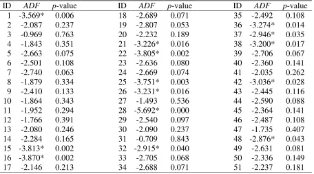
As a preliminary analysis, we implement the ADF test for relative commodity
prices (see Table 2).9 The test rejects the null of nonstationarity for only 14 out of 51
relative commodity prices at the 5% significance level. We are cautious in interpreting this
as an evidence for overall nonstationary, because the ADF test suffers from low power in
small samples. Panel unit root tests are one way to address the low power problem of
univariate tests. However, first-generation panel unit root tests, among others, Maddala
and Wu (1999), Levin et al. (2002), and Im et al. (2003), are known to be seriously
over-sized (reject the null hypothesis too often) when the true data generating process has
substantial cross-section dependence.
To see whether this is the case, we employ a cross-section dependence test by
Pesaran (2004),
(6)
where is the pair-wise correlation coefficients from the residuals of the ADF
regressions. The test rejects the null of no cross-section dependence at any conventional
9
significance level (see Table 2), which implies that first-generation panel tests are not
proper tools for our purpose.10
Table 2 around here
We next implement PANIC for the commodity prices. We first use and
criteria suggested by Bai and Ng (2002) to determine the number of common factors.
All criteria except choose two factors ( , see Figure 1).11
Applying the method of principal components as described in previous section, we
obtained the estimates for common factors factor loadings ( , and idiosyncratic
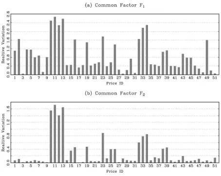
components ( ). We evaluate the importance of common factors for dynamics of the
commodity prices relative to idiosyncratic components by
(7)
where σ(·) denotes the standard deviation. As can be seen in Figure 2, dynamics of
individual commodity prices is substantially governed by the first common factor. For
many prices, is greater than one, which means that the first factor is more important
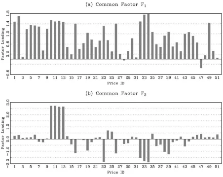
than idiosyncratic components for those prices. The second common factor also plays an
important role for some commodities such as crude oil prices. Similar evidence can be
found in factor loading estimates (Figure 3).
10
All results including individual correlation coefficients used in constructing the CD test statistic are available upon request.
11
Figures 1 through 3 around here
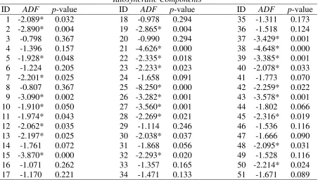
The PANIC unit root test results are reported in Table 3. The ADF test cannot
reject the null of nonstationarity for the first factor ( , but can reject the null for the
second factor at the 5% significance level.12 Since there is one nonstationary factor
among two common factors, , we do not implement cointegration tests.
For the de-factored (filtered) idiosyncratic components, the ADF test rejects the null for 29
out of 51 relative commodity prices. The panel unit root test by (5) rejects the null
hypothesis at any common significance level. The results given here provide strong
evidence that there is a single nonstationary common factor that drives the persistent
movement of commodity prices.
Table 3 around here
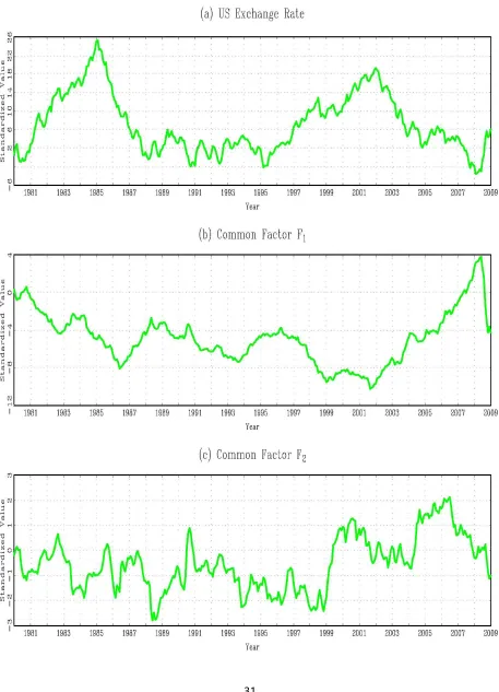
Since the factors are latent variables, there is no obvious way of identifying the
source of this nonstationarity. However, we note that the estimated first common factor is
approximately a mirror image of the US nominal exchange rate (see Figure 4). The
exchange rate exhibits two big swings in 1980s and from mid 1990s until mid 2000s. We
note that the first common factor estimate exhibits similar big swings in opposite
directions. This may make sense when we recognize most commodities are priced in US
12
dollars. When the US dollar depreciates relative to overall other currencies, nominal
commodity prices may rise given the world price, and vice versa. Because aggregate prices
such as the CPI tend to exhibit sluggish movements with low volatility, relative commodity
prices exhibit upward movements.
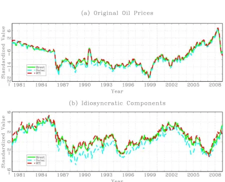
The second common factor shows stable fluctuations which may be consistent with
stationarity.13 Figure 5 provides some interesting dynamics of three crude oil prices, that is,
Brent, Dubai, and Western Texas Intermediate oil prices. We plot oil prices in panel (a)
while de-factored oil prices (idiosyncratic components) are drawn in panel (b). Panel (a)
clearly shows extremely persistent (possibly nonstationary) movements of oil prices.
De-factored oil prices, however, exhibit much less persistent dynamics.
The economic profession seems to agree on the nonstationarity of nominal
exchange rates. If so, and if commodity prices are largely governed by a single
nonstationary common factor, it is not unreasonable to suggest that such nonstationarity is
inherited from the US nominal exchange rate. The remaining factors and/or idiosyncratic
components may reflect changes in world demand and supply conditions, which may
fluctuate around the long-run equilibrium in accordance with price theories.
Figures 4 and 5 around here
To further investigate the link between commodity prices and the value of the US
dollar, we implement out-of-sample forecast exercises based on our factor model, with the
13
random walk model serving as a benchmark.14 We use a conventional method proposed by
Diebold and Mariano (1995) and West (1996) to evaluate the out-of-sample forecast
accuracy of these models.
Let denote the natural logarithm US nominal exchange rate. The random walk
model of implies
, (8)
where is the k-step ahead forecast by the random walk model given information set
at time t. The competing model using the two common factors from the commodity price
panel is based on the following least squares regression
. (9)
Given the least squares coefficient estimate, we construct the k-step ahead forecast by the
factor model by
, (10)
where is the fitted value from (9) and is the actual data at time t. Note that
conditional forecasts for the return (differenced) variables for as well as the
current period level variable are iteratively used to get the -period ahead conditional
forecast for the level exchange rate.
The forecast errors from the two models are,
14
For the Diebold-Mariano-West test, define the following function.
) – ,
where ), is a loss function.15 To test the null of equal predictive accuracy,
: , the Diebold-Mariano-West statistic (DMW) is defined as
(11)
where is the sample mean loss differential,
,
is the asymptotic variance of ,
,
(·) denotes a kernel function where (·) = 0, , and is the autocovariance
function estimate.16 It is known that the DMW statistic is severely under-sized with
asymptotic critical values when competing models are nested, which is the case here. We
use critical values by McCracken (2007) to avoid this size distortion problem.
15
We use the conventional squared error loss function,
16
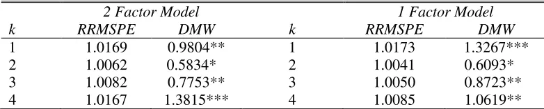
To further address the possibility that the first common factor measures the effect of
the exchange rate on commodity prices, we report out-of-sample forecast exercise results in
Table 4. We carried out forecasting recursively by sequentially adding one additional
observation from 180 initial observations toward 360 total observations for forecast
horizons ranging = 1, 2, 3, 4. First, the ratios of the root mean square prediction error of
the random walk model to the factor model were greater than one for all , that is, the
factor model outperformed the benchmark random walk model. Second, the DMW
statistics with McCracken’s (2007) critical values rejects the null of equal predictability for
= 1, 4 at the 5% significance level and for = 3 at the 10% level when estimated factors
from nominal prices are used. Using factors from relative prices, we obtain even stronger
evidence of forecast predictability.17
Table 4 around here
4
Concluding Remarks
We began this paper by noting a dichotomy between the implications of economic theory
concerning the dynamic behavior of commodity prices and the implications of empirical
tests of that behavior: stable commodity market equilibria should imply some form of
stationary (mean reverting) commodity price behavior over time, but unit root tests on the
behavior of commodity prices typically find evidence of nonstationarity. To investigate
17
this dichotomy, we undertook a careful analysis of what factors play dominant roles in
determining the dynamics of highly tradable commodity prices. Employing the PANIC
method of Bai and Ng (2004), we identified two important common factors from 51 world
relative commodity prices.
The first common factor explains the largest proportion of the variation in the panel
of prices. It was found to be nonstationary, and there is theoretical, graphical, and out of
sample forecasting evidence that it is closely related to the nominal US exchange rate. The
result that our simple two-factor model significantly outperforms a random walk in
forecasting the exchange rate is itself of interests, because the profession has recognized
that the random walk model consistently outperforms economic models for forecasting the
exchange rate since the work of Meese and Rogoff (1983).
One is tempted to suggest that this factor measures the effect of the exchange rate
on our panel of commodity prices. But perhaps a more appropriate inference is that this
factor and exchange rates share information content; factors that have a predictable effect
on the exchange rate will have a correspondingly predictable effect on commodity prices.
The second common factor and the idiosyncratic components of each series were
found to be stationary. Results for these components are consistent with equilibrium price
dynamics – short-lived deviations that quickly revert back to equilibrium. Thus, when the
effects of the exchange rate, or at the minimum the first common factor, are filtered out of
the panel of commodity prices, the remaining factors affecting commodity prices exhibit
Taken together these two results provide a viable rationale for the theory/evidence
Reference
1. Andrews, Donald W.K. and J. Christopher Monahan. 1992. An improved
heteroskedasticity and autocorrelation consistent covariance matrix estimator.
Econometrica, 60(4), pp. 953-66.
2. Ardeni, Pier Giorgio. 1989. Does the law of one price really hold for commodity
prices? American Journal of Agricultural Economic Association, 71(3), pp.
661-669.
3. Babula, Ronald A., Fred J. Ruppel, and David A, Bessler. 1995. U.S. corn exports:
the role of the exchange rate. Agricultural Economics, 13, pp. 75-88.
4. Bai, Jushan and Serena Ng. 2002. Determining the number of factors in
approximate factor models. Econometrica, 70(1), pp. 191-221.
5. Bai, Jushan and Serena Ng. 2004. A PANIC attack on unit roots and cointegration.
Econometrica, 72(4), pp. 1127-1177.
6. Balagtas, Joseph V. and Matthew T. Holt. 2009. The commodity terms of trade,
unit roots, and nonlinear alternatives: a smooth transition approach. American
Journal of Agricultural Economics, 91(1), pp. 87-105.
7. Chen, Yu-chin, Kenneth Rogoff, and Barbara Rossi. 2010. Can exchange rates
forecast commodity prices? Quarterly Journal of Economics, 125(3), 1145-1194.
8. Diebold, Francis X. and Roberto S. Mariano. 1995. Comparing predictive
9. Enders, Walter and Matthew T. Holt. 2012. Sharp break or smooth shifts? An
investigation of the evolution of primary commodity prices. American Journal of
Agricultural Economics, 94(3), pp. 659-673.
10.Engel, Charles and John H. Rogers. 2001. Violating the law of one price: should
we make a federal case out of it. Journal of Money, Credit, and Banking, 33(1),
pp.1-15.
11.Goodwin, Barry K. 1992. Multivariate cointegration tests and the law of one price
in international wheat markets. Review of Agricultural Economics, 14(1), pp.
117-24.
12.Goodwin, Barry K., Matthew T. Holt and Jeffrey P. Prestemon. 2011. North
American oriented strand board markets, arbitrage activity, and market price
dynamics: a smooth transition approach. American Journal of Agricultural
Economics, 94(3), pp. 993-1014.
13.Gospodinov, Nikolay and Serena Ng. 2010. Commodity prices, convenience yields
and inflation. mimeo.
14.Groen, Jan J. J. and Paolo A. Pesenti. 2010. Commodity prices, commodity
currencies, and global economic development. NBER Working Papers, 15743.
15.Holt, Matthew T. and Lee A. Craig. 2006. Nonlinear dynamics and structural
change in the U.S. hog-corn cycle: a time-varying STAR approach. American
Journal of Agricultural Economics, 88(1), pp. 215-233.
16.Im, Kyung So, M. Hashem Pesaran, and Yongcheol Shin. 2003. Testing for unit
17.Isard, Peter. 1977. How far can we push the “law of one price”? American
Economic Review, 67(5), pp.942-48.
18.Kellard, Neil and Mark E. Wohar. 2006. On the prevalence of trends in primary
commodity prices. Journal of Development Economics, 79(1), pp. 146-67.
19.Larson, Arnold B. 1964. The hog cycle as harmonic motion. American Journal of
Agricultural Economics, 46(2), pp. 375-386.
20.Levin, Andrew, Chien-Fu Lin, and Chia-Shang James Chu. 2002. Unit root tests in
panel data: asymptotic and finite sample properties. Journal of Econometrics,
98(1), pp. 1-24.
21.Lo, Ming Chien and Eric Zivot. 2001. Threshold cointegration and nonlinear
adjustment to the law of one price. Macroeconomic Dynamics, 5(4), pp. 533-76.
22.Maddala, G. S. and Shaowen Wu. 1999. A comparative study of unit root tests with
panel data and a new simple test. Oxford Bulletin of Economics and Statistics,
Special Issue v.61, pp. 631-52.
23.McCracken, Michael W. 2007. Asymptotics for out of sample tests of Granger
causality. Journal of Econometrics, 140(2), pp. 719-52.
24.Meese, Richard and Kenneth Rogoff. 1982. The out-of-sample failure of empirical
exchange rate models: sampling error or misspecification? International Monetary
Fund’s International Finance Discussion Papers, 204.
25.Michael, Panos, A. Robert Nobay, and David Peel. 1994. Purchasing power parity
yet again: evidence from spatially separated commodity markets. Journal of
26.Moon, Hyungsik Roger and Benoit Perron. 2004. Testing for a unit root in panels
with dynamic factors. Journal of Econometrics, 122(1), pp. 81-126.
27.Ng, Serena and Pierre Perron. 1995. Unit root tests in ARMA models with
data-dependent methods for the selection of the truncation lag. Journal of the American
Statistical Association, 90, pp. 268-281.
28.Mundlak, Yair and He Huang. 1996. International comparisons of cattle cycles.
American Journal of Agricultural Economics, 78(4), pp. 855-868.
29.Obstfeld, Maurice and Alan M. Taylor. 1997. Nonlinear aspects of good-market
arbitrage and adjustment: Heckscher’s commodity points revisited. NBER Working
Papers, 6053.
30.Parsley, David C. and Shang-Jin Wei. 2001. Explaining the border effect: the role
of exchange rate variability, shipping costs, and geography. Journal of
International Economics, 55(1), pp. 87-105.
31.Pesaran, M. Hashem. 2004. General diagnostic tests for cross section dependence
in panels. CESIFO Working Paper, 1229.
32.Pesaran, M. Hashem. 2007. A simple panel unit root test in the presence of
cross-section dependence. Journal of Applied Econometrics, 22(2), pp. 265-312.
33.Phillips, Peter C. B. and Donggyu Sul. 2003. Dynamic panel estimation and
homogeneity testing under cross section dependence. Econometrics Journal, 6(1),
34.Sarno, Lucio, Mark P. Taylor, and Ibrahim Chowdhury. 2004. Nonlinear dynamics
in deviations from the law of one price: a broad-based empirical study. Journal of
International Money and Finance, 23(1), pp. 1-25.
35.Stock, James H. and Mark W. Watson. 2002. Forecasting using principal
components from a large number of predictions. Journal of the American Statistical
Association, 97, pp. 1167-1179.
36.Wang, Dabin and William G. Tomek. 2007. Commodity prices and unit root tests.
American Journal of Agricultural Economics, 89(4), pp. 873-889.
37.West, Kenneth D. 1996. Asymptotic inference about predictive ability.
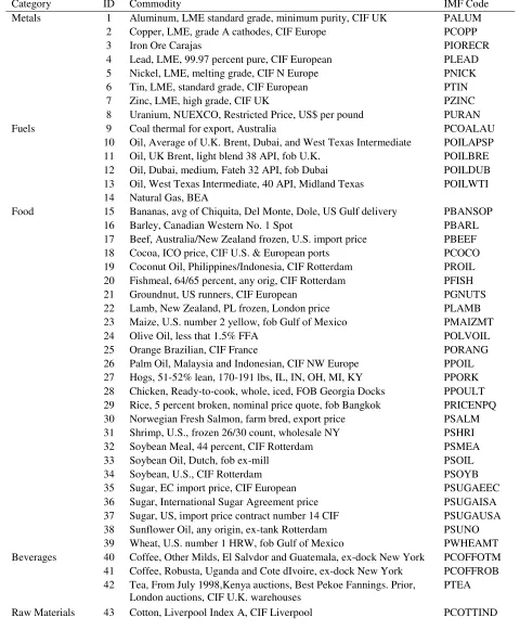
Table 1. Commodity Price Data Description
Category ID Commodity IMF Code
Metals 1 Aluminum, LME standard grade, minimum purity, CIF UK PALUM 2 Copper, LME, grade A cathodes, CIF Europe PCOPP
3 Iron Ore Carajas PIORECR
4 Lead, LME, 99.97 percent pure, CIF European PLEAD 5 Nickel, LME, melting grade, CIF N Europe PNICK 6 Tin, LME, standard grade, CIF European PTIN 7 Zinc, LME, high grade, CIF UK PZINC 8 Uranium, NUEXCO, Restricted Price, US$ per pound PURAN Fuels 9 Coal thermal for export, Australia PCOALAU
10 Oil, Average of U.K. Brent, Dubai, and West Texas Intermediate POILAPSP 11 Oil, UK Brent, light blend 38 API, fob U.K. POILBRE 12 Oil, Dubai, medium, Fateh 32 API, fob Dubai POILDUB 13 Oil, West Texas Intermediate, 40 API, Midland Texas POILWTI 14 Natural Gas, BEA
Food 15 Bananas, avg of Chiquita, Del Monte, Dole, US Gulf delivery PBANSOP 16 Barley, Canadian Western No. 1 Spot PBARL 17 Beef, Australia/New Zealand frozen, U.S. import price PBEEF 18 Cocoa, ICO price, CIF U.S. & European ports PCOCO 19 Coconut Oil, Philippines/Indonesia, CIF Rotterdam PROIL 20 Fishmeal, 64/65 percent, any orig, CIF Rotterdam PFISH 21 Groundnut, US runners, CIF European PGNUTS 22 Lamb, New Zealand, PL frozen, London price PLAMB 23 Maize, U.S. number 2 yellow, fob Gulf of Mexico PMAIZMT 24 Olive Oil, less that 1.5% FFA POLVOIL 25 Orange Brazilian, CIF France PORANG 26 Palm Oil, Malaysia and Indonesian, CIF NW Europe PPOIL 27 Hogs, 51-52% lean, 170-191 lbs, IL, IN, OH, MI, KY PPORK 28 Chicken, Ready-to-cook, whole, iced, FOB Georgia Docks PPOULT 29 Rice, 5 percent broken, nominal price quote, fob Bangkok PRICENPQ 30 Norwegian Fresh Salmon, farm bred, export price PSALM 31 Shrimp, U.S., frozen 26/30 count, wholesale NY PSHRI 32 Soybean Meal, 44 percent, CIF Rotterdam PSMEA 33 Soybean Oil, Dutch, fob ex-mill PSOIL 34 Soybean, U.S., CIF Rotterdam PSOYB 35 Sugar, EC import price, CIF European PSUGAEEC 36 Sugar, International Sugar Agreement price PSUGAISA 37 Sugar, US, import price contract number 14 CIF PSUGAUSA 38 Sunflower Oil, any origin, ex-tank Rotterdam PSUNO 39 Wheat, U.S. number 1 HRW, fob Gulf of Mexico PWHEAMT Beverages 40 Coffee, Other Milds, El Salvdor and Guatemala, ex-dock New York PCOFFOTM
41 Coffee, Robusta, Uganda and Cote dIvoire, ex-dock New York PCOFFROB 42 Tea, From July 1998,Kenya auctions, Best Pekoe Fannings. Prior,
London auctions, CIF U.K. warehouses
44 Wool Coarse, 23 micron, AWEX PWOOLC 45 Wool Fine, 19 micron, AWEX PWOOLF Industrial Inputs 46 Hides, US, Chicago, fob Shipping Point PHIDE
Table 2. Augmented Dickey-Fuller Test and Cross-Section Dependence Test Results: Relative Commodity Prices
ID ADF p-value ID ADF p-value ID ADF p-value
1 -3.569* 0.006 18 -2.689 0.071 35 -2.492 0.108
2 -2.087 0.237 19 -2.807 0.053 36 -3.274* 0.014
3 -0.969 0.763 20 -2.232 0.189 37 -2.946* 0.035
4 -1.843 0.351 21 -3.226* 0.016 38 -3.200* 0.017
5 -2.663 0.075 22 -3.805* 0.002 39 -2.706 0.067
6 -2.501 0.108 23 -2.636 0.080 40 -2.360 0.141
7 -2.740 0.063 24 -2.669 0.074 41 -2.035 0.262
8 -1.879 0.334 25 -3.751* 0.003 42 -3.036* 0.028
9 -2.410 0.133 26 -3.231* 0.016 43 -2.445 0.116
10 -1.864 0.343 27 -1.493 0.536 44 -2.590 0.088
11 -1.952 0.294 28 -5.692* 0.000 45 -2.364 0.141
12 -1.766 0.391 29 -2.540 0.097 46 -2.487 0.108
13 -2.080 0.246 30 -2.090 0.237 47 -1.735 0.407
14 -2.284 0.165 31 -0.709 0.843 48 -2.876* 0.043
15 -3.813* 0.002 32 -2.915* 0.040 49 -2.631 0.081
16 -3.870* 0.002 33 -2.705 0.068 50 -2.336 0.149
17 -2.146 0.213 34 -2.688 0.071 51 -2.237 0.181
CD Statistic: 48.313*, p-value: 0.000
Table 3. PANIC Test Results: Relative Commodity Prices
Idiosyncratic Components
ID ADF p-value ID ADF p-value ID ADF p-value
1 -2.089* 0.032 18 -0.978 0.294 35 -1.311 0.173
2 -2.890* 0.004 19 -2.865* 0.004 36 -1.518 0.124
3 -0.798 0.367 20 -0.990 0.294 37 -3.429* 0.001
4 -1.396 0.157 21 -4.626* 0.000 38 -4.648* 0.000
5 -1.928* 0.048 22 -2.335* 0.018 39 -3.385* 0.001
6 -1.224 0.205 23 -2.233* 0.023 40 -2.078* 0.033
7 -2.201* 0.025 24 -1.658 0.091 41 -1.773 0.070
8 -0.807 0.367 25 -8.250* 0.000 42 -2.259* 0.022
9 -3.090* 0.002 26 -3.282* 0.001 43 -3.578* 0.001
10 -1.910* 0.050 27 -3.560* 0.001 44 -1.802 0.066
11 -1.974* 0.043 28 -2.269* 0.021 45 -2.316* 0.019
12 -2.062* 0.035 29 -1.114 0.246 46 -1.536 0.116
13 -2.197* 0.025 30 -2.038* 0.037 47 -1.666 0.090
14 -1.761 0.072 31 -1.868 0.056 48 -2.095* 0.031
15 -3.870* 0.000 32 -2.293* 0.020 49 -1.528 0.116
16 -1.071 0.262 33 -1.357 0.165 50 -2.214* 0.024
17 -1.170 0.221 34 -1.471 0.133 51 -1.671 0.089
Panel Test Statistics: 19.497*, p-value: 0.000
Common Factor Components
ADF (Factor 1): -1.887, p-value; 0.326 ADF (Factor 2): -2.912*, p-value: 0.040
Note: i) ADF denotes the augmented Dickey-Fuller t-statistic with no deterministic terms (idiosyncratic
Table 4. Out-of-Sample Forecast Performance: Relative Commodity Price Factors
2 Factor Model 1 Factor Model
k RRMSPE DMW k RRMSPE DMW
1 1.0169 0.9804** 1 1.0173 1.3267***
2 1.0062 0.5834* 2 1.0041 0.6093*
3 1.0082 0.7753** 3 1.0050 0.8723**
4 1.0167 1.3815*** 4 1.0085 1.0619**
Note: i) Out-of-sample forecasting was recursively implemented by sequentially adding one additional observation from 180 initial observations toward 360 total observations. ii) k denotes the forecast horizon. iii) RRMSPE denotes the ratio of the root mean squared prediction error of the random walk hypothesis to the common factor model. iv)