Four Steps Continuous Method for the Solution of y″= f (x, y, y′)

(1)

Four Steps Continuous Method for the Solution of







, ,



y



f x y y

Adetola Olaide Adesanya1, Mattew Remilekun Odekunle1, Mfon Odo Udoh2*

1_{Department of Mathematics, Modibbo Adama University of Technology, Yola, Nigeria} 2_{Department of Mathematics and Statistics, Cross River State University of Technology, Calabar, Nigeria}

Email: torlar10@yahoo.com, remi_odekunle@yahoo.com, *_{mfudo4sure@yahoo.com}

Received January 5,2013; revised February 18, 2013; accepted March 30, 2013

Copyright © 2013 Adetola Olaide Adesanya et al. This is an open access article distributed under the Creative Commons Attribution License, which permits unrestricted use, distribution, and reproduction in any medium, provided the original work is properly cited.

ABSTRACT

This paper proposes a continuous block method for the solution of second order ordinary differential equation. Colloca-tion and interpolaColloca-tion of the power series approximate soluColloca-tion are adopted to derive a continuous implicit linear multistep method. Continuous block method is used to derive the independent solution which is evaluated at selected grid points to generate the discrete block method. The order, consistency, zero stability and stability region are investi-gated. The new method was found to compare favourably with the existing methods in term of accuracy.

Keywords: Predictor; Corrector; Collocation; Interpolation; Power Series Approximant; Continuous Block Method

1. Introduction

This paper considered the solution to the second order initial value problem of the form

   





 

0 0

, ,

y f x y x y x y x y

y x y

 

  

,



(1)

Predictor-corrector method for solving higher order ordinary differential equation has been proposed by many scholars. These authors are [1-5]. They individually pro-posed continuous implicit linear multistep method where separate reducing order of accuracy predictors was devel-oped and Taylor series expansion provided the starting value. The major setback of this method is the cost of developing predictors. Moreover, the predictors devel-oped are of lower order to the corrector; hence it has a great effect on the accuracy of the results.

In order to cater for the shortcoming of predictor-corrector method, scholars proposed block method. Block method gives solutions at each grid within the interval of integration without ovelapping and the burden of devel-oping separate predictors is eradicated. The authors who proposed block method are [6-12]. These authors pro-posed a discrete block method, which did not enable evaluation at all points within the interval of integration.

In this paper, we propose a continuous block method

which enables evaluation at all points within the interval of integration without starting the block all over. Con-tinuous block method enables one to recover discrete block when evaluating at selected grid points.

2. Methodology

Given the general block formulae proposed by [11]

 



.

m yn h yn h Ym

 

  

Y E DF BF





(2)

where m



n n n k T 1, 2, ,

y y y



Y  ,  is the order of the differential equation, K is the steplenght, ,E D and

are matrices. We then propose a prediction equation in the form

B

 0 2  

_{ }

0

.

m yn h y

   





 



Y E F _n (3)

where  

 



, ,



.

n



_y

y f x y y x

 



 _

 

F Substituting (3)

into (2) gives

 

 0

.

m yn h yn h B m

 

  

Y E DF F Y (4)

Equation (4) is non self starting since the prediction equation is not gotten directly from the block formulae as proposed by [13].

In formulating the continuous block method we now consider a continuous implicit linear multistep method given by

(2)

 

0 0

.

s r

n k k n k k n k

k k

Y_  x y_ h  x

 









f _ (5)

where s and are the numbers of interpolation and collocation points.

r

 

k x

 and k

 

x are polynomials.

Solving (5) for the independent solution gives a continuous block formulae in the form

 

_{ }

1

0 0

. !

m

r m

n j n j n k

j j

jh

Y y h x

m



 _ 

 

 









f (6)

where j

 

x is a polynomial, m1, 2, , 1. Evalu-

ating (6) at selected value of j reduces to (2).

Development of the Continuous Block Formula

Consider power series of a single variable as our ap-proximate solution in the form

 

1

0

.

s r j j j

y x a x

  





(7)

The second derivatives of (7) gives

 

1





2

0

1

s r

j j j

y x j j a x

 

 

 



 . (8)

putting (8) into (1) gives

   





1





2

0

, , s r 1 j

j j

.

f x y x y x j j a x

 

 

 



 (9)

Let the solution to (1) be soughted on the partition

0 1 with a

constant stepsize 2 1

πN:ax  x x xnxn x b



N



h given as

, 0,1, 2, ,

n i n

hx_ x n _ N.

1

Interpolating (7) at xn s ,s0, and collocating (9) at

gives

 

, 0 1 4

n r

x_ r

1

0

.

s r j j n r j

a x y

 

 





(10)





1

2 2

1

s r

j _.

j n r

j

j j a x f

 

  

 



(11)

solving (10) and (11) for a sj and substituting back in

(7) gives a continuous linear multistep method of the form

 

1

 

2 4

 

0 0

.

j n j j n j

j j

y x  x y h  x f

 







4

1 ₂ ₁₈ ₅₅ ₆₀ ₂₁

1440 t t t t t

      ;

where

.

n

x x

t h

 

3

1

2 21 70 80

360 t t t t

      ;



6 5 4 3



4

1 ₂ ₁₈ ₅₅ ₆₀

1440 t t t t

     ;

Evaluating the continuous block method at t1 1 4

 

gives a discrete block formulae of the form (2) where 0 0 0 1 0 0 0 1

0 0 0 1 0 0 0 2 0 0 0 1 0 0 0 3 0 0 0 1 0 0 0 4 , 0 0 0 0 0 0 0 1 0 0 0 0 0 0 0 1 0 0 0 0 0 0 0 1 0 0 0 0 0 0 0 1

 

 

  

 

 

E

T

367 53 147 56 251 29 27 14 _, 1440 90 160 45 720 90 80 45

 

 _ _

D

T

3 8 117 64 323 62 51 64 8 5 40 15 360 45 40 45

47 1 27 16 11 4 9 8

240 3 80 15 30 15 10 15 _,

29 8 3 64 53 2 21 64

360 45 8 45 360 45 40 45

7 1 9 ₀ 19 1 3 14

480 30 160 720 90 80 45

 

 

  

 

  

 

_ _ _ _ _ _ 

 

 

B

 0 _{ }_{8 8}

(3)

 





 

2

0 1 2

1 1 2 2

1 2

;

p p p

p p p p

p p

y x h

C y x C hy x C h y x C h y x

C _h  y  x C _ h  y  x

             (14)

3. Analysis of the Basic Properties of the

Corrector

3.1. Order of the Method

Let the linear operator 



y x h

 

;



associated with the

block formulae be defined as _{ated continuous linear multistep method}Definition 1.The linear operator and the associ-₍₁₃₎_{are said to} be of order p if 0 1 2 1



Cp p 0

C  c C  C   and

2 0.

p

C   Cp2 is called the error constant and implies

that the local truncation error is given by

 





 0

_{ }

;

.

m n n m

y x h

y h y h Y

A Y E  DF  BF



(13)

 2  2

_{ }

 

3

2 .

p p p

n k p n

t _ C _ h  y  x O h  (15)

expanding in Taylor series and comparing the coefficient

of h gives For our method,

 





1 2 3 2 4 1 2 3 4

367 3 47 29 7

1440 8 240 360 480

53 8 1 8 1

90 3 3 45 30

1 1 ₁₄₇ ₁₁₇ ₂₇ ₃ ₉

1 2 ₁₆₀ ₄₀ ₈₀ ₈ ₁₆₀

1 3 ₅₆ ₆₄ ₁₆ ₆₄

1 4 ₇₂₀ ₁₅ ₁₅

; 0 1 0 1 0 1 0 1 n n n n n n n n n n y y y y y

y x h h

y hy y y y                 _                _{  }      _  _ __        _     _           _ _    1 2 3 4 0 15 ₀

251 323 11 53 19 720 360 30 360 720

29 62 4 2 1

90 45 15 45 90

27 51 9 21 3

80 40 10 40 80

14 64 8 64 1

445 45 15 45 45

n n n n n f f f f f                    _{ } _  _{ } _  _{ } _  _ _    _{ } _  _{ } _  _  _ _      _           

Expanding in Taylor series gives

 

_{ }

 

_{ }

 

  2 2 2 2 0 0 2 2 2 2 0 0 2 2 2 0

367 3 47 29 7

1 2 3 4

! 1440 ! 8 240 360 480

2 ₂ 53 8 ₁ 1 ₂ 8 ₃ 1

! 90 ! 5 3 45 30

3 ₃ 147

! 160 !

j _j

j j j j

j j

n n n n n

j j

j _j

j j j j

j j

n n n n n

j j

j _j

j

n n n n

j

h h

y y hy h y y

j j

h h

y y hy h y y

j j

h h

y y hy h y

j j                       _    _                     



4

 

_{ }

 

_{ }

2 0 2 2 2 2 0 0 2 2 1 2 0 0

117 ₁ 27 ₂ 3 ₃ 9 ₄

40 80 8 160

4 ₄ 56 64 ₁ 16 ₂ 64 ₃

! 45 ! 15 15 45

251 323 ₁ 11 ₂ 53 ₃ 19 ₄

! 720 ! 360 30 360 720

j j j j

j n j

j _j

j j j

j j

n n n n n

j j

j _j

j j j j

j j

n n n n

j j

y

h h

y y hy h y y

j j

h h

y hy hy y

j j                  _ _ _                         _    _  



 

_{ }

 

_{ }

 

  2 2 1 2 0 0 2 2 1 2 0 0 2 2 1 2 0

2 ₂ 29 62 ₁ 4 ₂ 2 ₃ 1 ₄

! 90 ! 45 15 45 90

3 27 51 9 21 3

3 1 2 3 4

! 80 ! 40 10 40 80

4 14 64

4

! 45 !

j _j

j j j j

j j

n n n n

j j

j _j

j j j j

j j

n n n n

j j

j _j

j j

n n n n

j

h h

y hy hy y

j j

h h

y hy hy y

j j

h h

y hy hy y

j j                          _    _         _    _      



 

0 0

8 64 14

1 2 3 4

45 45 45 45

j j j j

(4)

hence,

0 1 2 3 4 5 6 7 0

C C C C C C C C 

8

107 8 9 16 3 1 3 8

10080 315 225 315 160 90 160 945

C    _

 

4. Zero Stability

Definition 2. The block (2) is said to be zero stable, if the roots of the first characteristic poly-nomial defined by satis-fies

, 1, 2, ,

s

z s _ N

 

z



 

_det



 0



z zA

 

the differential equation. Moreover as h0,

 

r



1 ,



z z  z 

 _  _

where  is the order of the dif- ferential equation, r is the order of the matrix and

E(see [11] for details).

 0

A

E

 1

s

z  have multiplicity not exceeding the order of For our method

 

1 0 0 0 0 0 0 0 0 0 0 1 0 0 0 1

0 1 0 0 0 0 0 0 0 0 0 1 0 0 0 2

0 0 1 0 0 0 0 0 0 0 0 1 0 0 0 3

0 0 0 1 0 0 0 0 0 0 0 1 0 0 0 4

0 0 0 0 1 0 0 0 0 0 0 0 0 0 0 1

0 0 0 0 0 1 0 0 0 0 0 0 0 0 0 1

0 0 0 0 0 0 1 0 0 0 0 0 0 0 0 1

0 0 0 0 0 0 0 1 0 0 0 0 0 0 0 1

z z



    

   

_{ } _{ }

   

 _  _{ }

 

0

                       

 

6



₁



2

z z z

   ; hence our method is zero stable.

Region of Absolute Stability

Definition 3. The method (2) is said be absolutely stable if for a given value oh h, all the roots zs of the

charac-teristic polynomial π

 

z h, 

 

z h

 

z 0, satis- fies zs 1,s1, 2, , n where

2 2_h



h  and f y

   .

do

We a pted the boundary locus method for the region of absolute stability if the block method. Substituting the test equation 2

y   y into the block formula gives

n

_{ }

 

n m

r y r

h r h

y r r

 

 _ _



 

A Y E

D BY



writing in trigonometric ratios gives

 

_, A Y 0

_{ }

m

 

  n

_{ }

 

_.

n m

h r

y

 



 _ _



 

Ey

D BY (16)

where _{e .}i

r  Equation (16) is our characteristics poly- (see [1

nomial 4] for details). Applying to our method

 

, 6975cos 4 6975

h r    _

168cos793

 

which gives the stability region to be [−14.35, 0] after evaluation h

 

,h at interval of 30 within [0, 180]

The stability is shown in Figure 1.

5. Numerical Experiments

5.1. Test Problems

We test our scheme on lems.

second order initial value

prob-.V.P) which was solved by [11] using block m

Problem 1: Consider the non linear initial value prob-lem (I

ethod and [2] for step size h0.003125 which is of

order 8

 

0,

 

0

 

1

y x y y 1, 0

2

y

   

Exact solution:

 

1 1 2

2 2

x

y x In

x



 

  _ _



[image:4.595.311.535.482.710.2]

 

Figure 1. Showing region of absolute stability of the bloc method.

(5)

We solved this problem using our method for stepsize h = 0.01. The result is shown in Table 1. Our method

performed better than the methods compared with. This problem method was also solved [10] using block of lower order for h = 1/32. Though the details are not shown but our result performed better in term of accu-racy.

Problem 2: Consider a linear second order initial value problem

 

2

6 4

y  y  y 0,y 1 1,y 1 1

x  x 

_{ } _ _   

   

Exact solution:

 

3 3

5 2

3 x y x

x

  .

[image:5.595.52.539.296.504.2]

This problem w b

Table 2 shows clearly that our method gives better

ap-proximation than the existing methods.

5.2. Numerical Results

The following notations are used in the table ESBK: Error in [11];

EAK: Error in [2]; EBK: Error in [10];

ERR Exact result computed result .

6. Conclusion

We have proposed a non self starting continuous block method in this paper. It has been shown clearly that the non self starting method gives a better approximation than as also solved y [10]. The result in

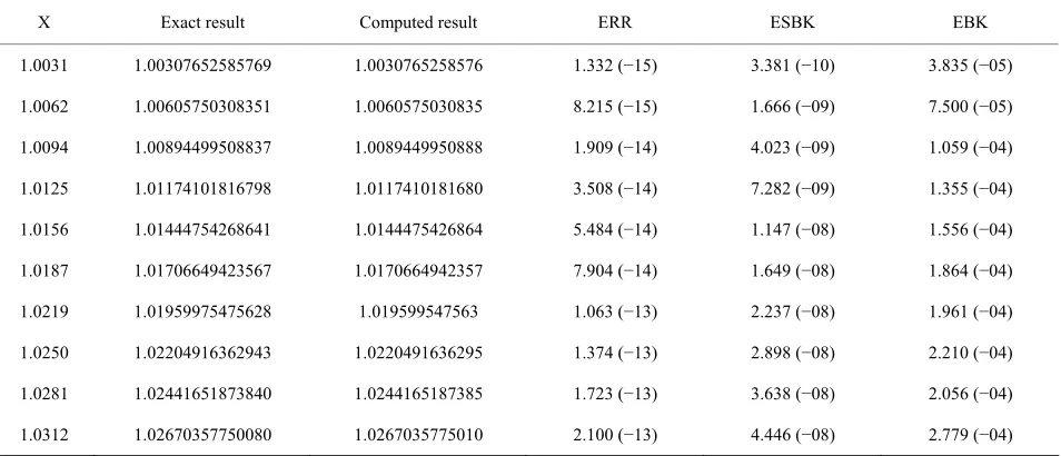
sults of problem 1.

X Exact result ESBK EAK

Table 1. Showing re

Computed result ERR

0.1 1.05004172927849 1.05004172927848 9.992 (−15) 6.442 (−11) 6.550 (−11) 0.2 1.10033534773107 1.10033534773099 8.149 (−14) 5.456 (−10) 5.480 (−10) 0.3 1.15114043593646 1.15114043593599 4.700 (−13) 1.921 (−09) 1.925 (−09) 0.4 1.20273255405408 1.20273255405244 1.637 (−12) 4.797 (−09) 4.802 (−09) 0.5 1.25541281188299 1.25541281187833 4.664 (−12) 9.998 (−09) 1.000 (−08) 0.6 1.30951960420311 1.30951960419194 1.116 (−11) 1.871 (−08) 1.872 (−08) 0.7 1.36544375427139 1.36544375424638 2.501 (−11) 3.272 (−08) 3.274 (−08) 0.8 1.43264893019360 1.42364893014144 5.215 (−11) 5.479 (−08) 5.396 (−08) 0.9 1.48470027859405 1.48470027848636 1.076 (−11) 8.929 (−08) 8.800 (−08) 1.0 1.54930614433405 1.54930614411698 2.170 (−10) 1.434 (−07) 1.435 (−07)

esults of proble

[image:5.595.61.538.531.736.2]

X Exact result ESBK EBK

Table 2. Showing r m 2.

Computed result ERR

(6)

the self starting ontinuo -troduced in the block method allows evaluation at all

o hin th ration; s

emi, “A New Sixth Order-Order Algorithm for the General Second Order Ordinary Differential Equa-tion,” Interna uter Mathematics

method. The c us parameter in

p ints wit e interval of integ hence, it enable researchers to understand the behaviour of the system under investigation. We therefore recommend this new method when seeking for the solution of initial value problems.

REFERENCES

[1] D. O. Awoy

tional Journal of Comp , Vol. 77, No. 1, pp. 117-124.

doi:10.1080/00207160108805054

[2] D. O. Awoyemi and S. J. Kayode, “A Maximal Order Collocation Method for Direct Solution of Initial Value Problems of General Second Orde

Equation,” Proceedings of the Con

r Ordinary Differential ference Organised by the National Mathematical Centre, Abuja, 2005.

[3] S. O. Adee, P. Onumanyi, U. V. serisena and Y. A. Ya-haya, “A Note on Starting Numerov’s Method More Ac-curately by an Hybrid Formula of Order Four for an Ini-tial Value Problem,” Journal of Computational and Ap-plied Mathematics, Vol. 175, No. 4, 2005, pp. 269-273. [4] D. O. Awoyemi and M. O. Idowu, “A Class of Hybrid

Collocation Method for Third Order Ordinary Differential Equation,” International Journal of Computer Mathe-matics, Vol. 82, No. 10, 2005, pp. 1287-1293.

doi:10.1080/00207160500112902

[5] A. O. Adesanya, T. A. Anake and M. O. Udoh, “Im-proved Continuous Method for Direct Solution of General Second Order Ordinary Differential Equations

of Nigerian Association of Mathem

,” Journal atical Physics, Vol. 13, 2008, pp. 59-62.

[6] S. N. Jator, “A Sixth Order Linear Multistep Method for Direct Solution of y f x y y



, , 



,” International

Jour-nal of Pu pp. 457-472

re and Ap atics, Vo .

[7] or and J. Starting istep

plied Mathem l. 40, No. 1, 2007, S. N. Jat Li, “A Self Linear Mult Method for the Direct Solution of the General Second Order Initial Value Problems,” International Journal of Computer Mathematics, Vol. 86, No. 5, 2009, pp. 817- 836. doi:10.1080/00207160701708250

[8] R. D’Ambrosio, M. Ferro and B. Paternoster, “Two-Steps Hybrid Method for y  f x y

 

, ,” Journal of Applied Mathematics Letters, Vol. 22, No. 7, 2009, pp. 1076-1080.

doi:10.1016/j.aml.2009.01.017

[9] I. Fudziah, H. K. Ya and O. Mohamad, “Explicit and Implicit 3-Point Block Method for Solving Special Sec-ond Order Ordinary Differential Equation Directly,” In-ternational Journal of Mathema

p

tical Analysis, Vol. 3, No. 5, 2009, pp. 239-254.

[10] Y. A. Yahaya and A. M. Badmus, “A Class of Colloca-tion Methods for General Second Order Differential Equa-tion,” African Journal of Math and Computer Research, Vol. 2, No. 4, 2009, pp. 69-71.

[11] D. O. Awoyemi, E. A. Adebile, A. O. Adesanya and T. A. Anake, “Modified Block Method for the Direct Solution of Second Order Ordinary Differential Equation,” Inter-national Journal of Applied Mathematics and Computa-tion, Vol. 3, No. 3, 2011, pp. 181-188.

[12] S. Mehrkanoon, “A Direct Variable Step Block Multistep Method for Solving General Third Order ODEs,” Journal of Numerical Algorithms, Vol. 57, No. 1, 2011, pp. 53-66.

doi:10.1007/s11075-010-9413-x

[13] S. Abbas, “Derivation of a new Block Method Similar to the Block Trapezoidal Rule for the Numerical Solution of First Order IVPs,” Science Echoes, Vol. 2, 2006, pp. 10- 24.