Munich Personal RePEc Archive
New financial intermediary development
indicators for developing countries
Simplice A., Asongu
HEC-Management School-University of Liège(Belgium)
15 May 2011
Online at
https://mpra.ub.uni-muenchen.de/38333/
New financial intermediary development indicators for developing
countries
Simplice A. Asongu
E-mail: [email protected]
Tel: 0032 473613172
HEC-Management School, University of Liège.
New financial intermediary development indicators for developing
countries
Abstract
Financial development indicators are often applied to countries/regions without taking
into account specific financial development realities. Financial depth in the perspective of
monetary base is not equal to liquid liabilities in every development context. This paper
introduces complementary indicators to the existing Financial Development and Structure
Database (FDSD) and unites two streams of research. It contributes at the same time to the
macroeconomic literature on measuring financial development and responds to the growing
field of economic development by means of informal financial sector promotion and
microfinance. The paper suggests a practicable way to disentangle the effects of the various
financial sectors on economic developments.
JEL Classification: E00; E26
1. Motivation
Financial development indicators have been universally applied without taking into
account regional/country specific financial development needs and realities. Usage of some
indicators for instance is based on the presumption that they are generally valid (Gries et al.,
2009)1; not withstanding empirical evidence that not all indicators may matter in financial
development (Asongu, 2010a). Furthermore, the absence of a consensus on the superiority of
financial development indicators; especially the widely used proxy for financial depth (Gries
et al., 2009) is desirous of research attention. As far as we have perused related literature, we
suppose that the absence of any study that focuses on the quality of financial development
indicators with respect to contextual development concerns is enough inspiration to search for
the missing link. It is therefore our objective in this paper to verify the validity of the financial
depth indicator as applied to developing countries and hence decompose it to new measures
that best address financial development challenges in developing countries. The underlying
impetus of our study is the misleading assumption that liquid liabilities can be proxied by the
monetary base (financial depth) in developing countries. This paper will therefore suggest a
practicable way to disentangle the effects of the various financial sectors on economic
developments. We shall develop testable hypotheses and propositions for more refined
financial development indicators and empirically verify their validity in the finance-growth
nexus. GDP and Monetary-base oriented ratios are developed for each sector of the financial
system. Our conception of the financial system goes beyond the realm of that expressed in the
International Financial Statistics’ definition; it integrates the informal sector, hitherto a
missing component in the existing measurement of the monetary base (M2).
Specific contributions of this paper to finance-growth literature include testing if: (1)
the informal financial sector significantly contributes to economic growth; (2) disentangling
1 Gries et al. (2003) state: “In the related literature several proxies for financial deepening have been suggested,
different components of the existing measurement could influence policy decisions and; (3)
introducing measures of sector importance to complement GDP ratio indicators could
ameliorate understanding of the finance-growth nexus.
Our study could be interesting to policy makers and researchers because it unites two
streams of research. It contributes at the same time to the macroeconomic literature on
measuring financial development and responds to the growing field of economic development
by means of informal financial sector promotion and microfinance. The absence of sound
fundamentals in a financial indicator might bias estimations and result in unhealthy policy
recommendations. The rest of the paper is structured in the following manner: section two
examines related literature and resulting hypotheses; new indicators based on testable
hypotheses are proposed in section three; data and methodology are presented and outlined
respectively in section four; section five focuses on empirical analysis; we conclude in section
six.
2. Related Literature
2.1 Monetary base as a biased indicator of liquid liabilities in developing countries
2.1.1 Definition of key-terms
a) Monetary Base
This is the amount of money in an economy. This is the measure of the money supply
that typically includes most liquid currencies. Measures of money are classified as level of M,
with the monetary base (M0) being the smallest and lowest M-level. While base money can
be described as the most acceptable liquid form of final payment, a broad measures of money
supply (M1) includes demand deposits to M0. Less liquid savings accounts such as time
deposits add up to M1 to define a broader money supply (M2). Large time deposits,
sum up to M2 to constitute the broadest money supply (M3). With respect to the context of
our paper M2 is more appropriate due to relative undeveloped financial sector of developing
countries. In the less developed world M0 could be assimilated to the informal financial
sector, implying the monetary base (M0) for the most part entails informal finance. As earlier
outlined, when formal and semi-formal banking sector deposits are integrated to M0 then a
broad money supply definition (M2) is obtained. Liquid liabilities should therefore be the
component of M2 circulating within the banking system (M2-M0).
b) Liquid liabilities
A Liquid liability is a debt or claim that has been converted into cash as it becomes
due. In the context of our work, it refers to bank deposits in current and savings accounts
(M2-M0). While in developed countries liquid liabilities could be assimilated to M2 (as M0 is
mostly held by the banking sector), in underdeveloped countries M0 quite often does not
transit through the banking sector and thus by definition is not a bank liability.
c) Financial system by International Financial Statistics (IFS)
According to the IFS, the financial system consists of deposit money banks (formal
banking sector) and other financial institutions (semi-formal banking sector)2. This definition
is ideal for developed countries (where M0 is part of the banking sector) but lacking in some
substance in the underdeveloped world (where most holders of liquidity contained in M0
don’t have bank accounts). Therefore according to this definition, financial depth is M2
without informal finance.
Within the framework of this paper financial depth corresponds to M2 (including the
informal financial sector)
2
2.1.2 Theoretical basis
Liquid liabilities expressed in terms of monetary base are without distinction of
financial sectors and rest on the assumption that almost all currency held is linked to a
financial sector deposit. Beck et al., (1999) on presenting a new database on financial
development and structure pointed-out: “Since many researchers have focused on the liability
side of the balance sheet, we include a measure of absolute size based on liabilities. Liquid
liabilities to GDP equal currency plus demand and interest-bearing liabilities of banks and
other financial intermediaries divided by GDP. This is the broadest available indicator of
financial intermediation, since it includes all three financial sectors....Liquid liability is a
typical measure of financial depth and thus the overall size of the financial sector without
distinguishing between financial sectors of the use of liabilities”(page 11). It is worth
emphasizing that almost no distinction is made between different financial sectors in the
FDSD; and the hypothesis of all constituents of the monetary base linked to the liability side
of the balance sheet is questionable for developing countries. Almost all currency held for
transaction motives in developed countries are still recycled in banks3. However, this is
subject to controversy in the underdeveloped world and therefore distinction between formal,
semi-formal and informal banking sectors is imperative.
A bias in the definition of financial system deposits (aka liquid liabilities) by the
International Monetary Fund (IMF) is deserving of examination. According to International
Financial Statistics (hence IFS), the financial system is made up of the formal and
semi-formal sectors; that is deposit money banks and other financial institutions (see lines 24, 25
and 45 of IFS, October 2008). While this definition could be quasi-true for developed
countries, it fails to take account of the informal financial sector in developing and
underdeveloped countries. This leaves us with some concern over the role of the informal
sector in financial intermediary development and growth.
3
2.1.3 Empirical framework
Though the monetary base (M2/GDP) which represents the money stock has been
widely used as a standard measure of liquid liabilities in many studies (World Bank 1989;
King and Levine, 1993), in developing countries a large part of the monetary base stock
consists of currency held outside banks. As such, an improvement in the M2/GDP ratio may
reflect an extensive use of currency rather than an increase in bank deposits. In an attempt to
curtail this shortcoming, Demetriades and Hussein (1996) suggested the subtraction of
currency outside banks from M2 in the measure of liquidity liabilities in developing countries.
Abu-Bader and Abu-Qarn (2008) amongst others have recently adjusted M2 in like manner.
But these adjustments fail to point-out that the “adjusted-measure “constitutes the formal and
semi-formal financial sectors. More so, the informal financial sector is ruled-out as marginal
in this conception of the finance-growth nexus. We shall endeavor to address these
insufficiencies in this paper.
Some authors have sought to address the issue by determining a broad variable that is
indicative of financial depth. They use the first principal component of M2/GDP and a
combination of one or more financial indicators (Khumbhakar and Mavrotas, 2005; Ang and
McKibbin, 2007). By so doing they decrease the dimensionality of the set of variables without
losing much information on the one hand; and on the other hand decrease problems related to
the quality of M2 as a measure of liquid liabilities. The set-back of this approach to a solution
is that, more often financial depth is mixed with concepts of financial activity (private
domestic credit/GDP), financial size (deposit bank assets/central bank assets plus deposit
money assets), financial allocation efficiency(bank credit/bank deposits)…etc. The
contribution of this paper to the existing literature is to address this problem without
Despite the partial awareness of this challenge, literature is inundated with works on
financial development in developing countries that do not distinguish between components in
M2 held by banks and currency held outside of the formal financial sector. We argue that
probing the distinction between formal, semi-formal and informal banking sectors could be
interesting in mastering the finance-growth nexus.
2.2 Why the concept of ‘financial-intermediary-formalization’ is crucial in economic
development?
In Africa a very low percentage of households have access to formal financial
services4. The issue is further evident with low population densities, poor transport and
limited communications infrastructure; which inhibit formal financial intermediation. Even
where such services are available, small and medium size businesses, and low income
individuals could find it difficult meeting-up with eligibility criteria such as strict
documentation requirements and/or collaterals. Beside constraints of physical access and
eligibility, cost barriers in the form of high transaction fees or considerable minimum
requirements for savings-balances or loan-amounts present another stumbling block.
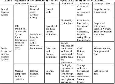
2.2.1 Distinction between formal, semi-formal and informal financial intermediaries
Firstly, as could be grasped from table 1 formal finance refers to services that are
regulated by the central bank and other supervisory authorities. Secondly, semi-formal finance
is a distinction between formal and informal finance. This is part of finance that occurs in a
formal financial environment but not formally recognized. An eloquent example is
micro-finance. Thirdly, informal finance is one that is not arranged through formal agreements and
not enforced through the legal system. The last two types of saving and lending are very
4
common in developing countries, particularly among the financially excluded or those on low
incomes.
Table 1 inspired by Steel (2006) clearly expatiates the role of semi-formal and
informal banks in the financial system of developing countries. Therefore, the role of Credit
Unions and Micro Finance NGOs (semi-formal finance) as well as elements of the last
[image:10.595.58.533.270.618.2]category cannot be undermined in the finance-led-growth nexus: such is the goal of our paper.
Table 1: Segments of the financial system by degree of formality in Paper’s context
Paper’s context Tiers Definitions Institutions Principal Clients
Formal financial system IMF Definition of Financial System from International Financial Statistics (IFS) Formal Financial sector (Deposit Banks) Formal banks Licensed by central bank Commercial and development banks Large businesses, Government Semi-formal and informal financial systems Semi-formal financial sector (Other Financial Institutions) Specialized non-bank financial institutions Rural banks, Post banks, Saving and Loan Companies, Deposit taking Micro Finance banks Large rural enterprises, Salaried Workers, Small and medium enterprises Other non-bank financial institutions Legally registered but not licensed as financial institution by central bank and government Credit Unions, Micro Finance NGOs Microenterprises, Entrepreneurial poor Missing component in IFS definition Informal financial sector Informal banks Not legally registered at national level(though may be linked to a registered association) Savings collectors, Savings and credit associations, Money lenders Self-employed poor Source (author)
2.2.2 Imperative of decomposing financial depth into formal, semi-formal and informal
components in financial intermediary development.
Hitherto, from a general macroeconomic perspective, the imperative of specifically
development has been marginal. We argue that stopping short of this would be gross injustice
to the two later categories (see table 1) which represent quite a significant bulk of the
financial sector in developing countries. The following stylized facts and hypotheses fully
express the spirit of decomposing financial depth into essential constituents.
a) Stylized facts
The IMF definition of the financial system is limited to the formal and semi-formal
sectors; that is deposits money banks and other financial institutions (see lines 24, 25 and 45
of International Financial Statistics, October 2008). While this could be quasi true for
developed countries, this definition holds less ground in developing and underdeveloped
worlds where, the informal financial sector takes a toll on the financial system and plays an
important role in economic growth and development.
Contrary to mainstream literature, in developing countries money in circulation plus
transaction and time deposits (M2) is not equal to liquid liabilities. This suggests that,
equating financial depth to liquid liabilities would be synonymous to assuming the inexistence
and/or insignificance of the informal financial sector. Money in circulation withheld by the
informal sector does not always transit through the banking system5. Therefore such currency
cannot be considered as formal bank sector deposits or liquid liabilities. More so, part of the
semi-formal financial sector made-up of other non-bank financial institutions that are legally
registered but not licensed as financial institutions by the central bank and government (e.g
Micro Finance NGO’s), also hold a substantial part of M2 which do not transit through
banking sector.
5
Besides introducing an informal financial sector indicator for growth, disentangling
the existing measure (M2) into its formal and semi-formal constituents in the context of
underdeveloped countries could improve our insight on the finance-growth nexus in the
growing field of financial and economic developments.
b) Testable hypotheses
Hypothesis 1: The informal financial sector (a previously missing component in the definition
of monetary base: M2) significantly contributes to economic growth.
Hypothesis 2: Disentangling different components of the existing measurement (financial
system) into formal (banking sector) and semi-formal (other financial institutions) financial
sector indicators could improve understanding of the finance-growth nexus.
Hypothesis 3: Introducing measures of sector importance could ameliorate the capacity to
understand how evolvements (improvements) of shares in different sectors of the financial
system affect the finance-growth nexus. To put this in other terms, the need to evaluate how
one financial sector develops at the expense of another and vice-versa could be crucial in
orienting policy-making.
Above hypotheses (with exclusive respect to components of M26) inspire propositions
on “financial development indicators” and “measures of sector importance”.
3. Propositions of new indicators
Financial development could either be indirect (financial intermediary development-
through the banking sector) or direct (through financial markets). The context of this study is
limited to the former type of financial development. Borrowing from Demirgüç-Kunt (1999),
6
indirect indicators could further be classified into financial development aspects of depth
(M2), allocation efficiency7, activity8 and size9. Amongst these measures, financial depth is
the most widely used in the finance-growth literature.
3.1 Financial development indicators (M2-based)
3.1.1 Formal financial development
Proposition 1: Formal financial development could be defined as:
GDP deposits Bank
op.1 _
Pr =
Bank deposits10 here refer to demand, time and saving deposits in deposit money banks.
3.1.2 Semi-formal financial development
Proposition 2: Semi-formal financial development could be appreciated as:
GDP
deposits Bank
deposits Financial
op.2 _ _
Pr = −
Financial deposits11 are demand, time and saving deposits in deposit money banks and other
financial institutions.
3.1.3 Informal financial development
Proposition 3: Informal financial development can be conceived as:
GDP deposits Financial M Base Monetary
op.3 _ ( 2) _
Pr = −
3.1.4 Informal and semi-formal financial development
Proposition 4: Informal and semi-formal financial development can be defined as:
GDP deposits Bank M Base Monetary
op.4 _ ( 2) _
Pr = −
7
Bank credit on bank deposits.
8
Private domestic credit on GDP.
9 Deposit bank assets / Central bank assets plus deposit bank assets. 10
Lines 24 and 25 of International Financial Statistics (IFS); October 2008.
11
3.2 Measures of sector importance
3.2.1 Financial intermediary formalization
Proposition 5: From ‘informal and semi-formal’ to formal financial development (formalization) ) 2 ( _ _ 5 . Pr M Base Monetary deposits Bank op =
In undeveloped countries M2 is not equal to liquid liabilities (liquid liabilities equal bank
deposits: bd). Whereas in undeveloped countries bd/M2<1, in developed countries bd/M2 is
almost equal to 1. This indicator measures the rate at which money in circulation is absorbed
by the banking system. Financial formalization here is defined as the propensity of the formal
banking system to absorb money in circulation.
3.2.2 Financial intermediary ‘semi-formalization’
Proposition 6: From ‘informal and formal’ to semi-formal financial development (Semi-formalization) ) 2 ( _ _ _ 6 . Pr M Base Monetary deposits Bank deposits Financial
op = −
This indicator measures the level at which the semi-formal financial sector evolves to
the detriment of formal and informal sectors.
3.2.3 Financial intermediary ‘informalization’
Proposition 7: From ‘formal and semi-formal’ to informal financial development (Informalisation) ) 2 ( _ _ ) 2 ( _ 7 . Pr M Base Monetary deposits Financial M Base Monetary
op = −
This proposition shows the rate at which the informal financial sector is developing at
Propositions 5, 6 and 7 add up to unity (one) arithmetically spelling-out the underlying
assumption of sector importance. That is, when their time series properties are considered in
empirical analysis, the evolution of one sector is to the detriment of other sectors and
vice-versa.
3.2.4 Financial intermediary ‘semi-formalization and informalization’
Proposition 8: Formal to ‘informal and semi-formal’ financial development: (Semi-formalisation and informalization)
) 2 ( _
_ )
2 ( _ 8
. Pr
M Base Monetary
deposits Bank
M Base Monetary
op = −
The proposition appreciates the deterioration of the formal banking sector to the
benefit of other sectors (informal and semi-formal). From common sense, proposition 5 and 8
should be perfectly antagonistic, meaning the former (formal financial development at the
expense of other sectors) and the later (formal sector deterioration) should display a perfectly
negative coefficient of correlation12.
3.2.5 Interaction of propositions
Owing to the compatibility of propositions 1, 2, 3 and 4 with propositions 5, 6, 7 and 8
respectively, we are poised to hypothesis that though the propositions are independent
significant determinants of growth, a combination of them would increase their effect on
growth (more than their independent sums). That is, for instance the combined of effect of
12
propositions 1 and 5(for formal finance) should be greater than the sum of independent effects
of propositions 1 and 5. The following testable hypothesis results there-from.
Hypothesis 4: For formal finance, simultaneous improvement of shares in GDP (Prop.1) and
Monetary Base (Prop.5) should have a higher impact on growth (than that expressed by their
independent sums). By the same token, this applies to semi-formal finance (Prop.2 and
Prop.6) and informal finance (Prop.3 and Prop.7).
3.2.6 Linkages between financial development measures, financial depth and liquid liabilities
Liquid liabilities are equal to the Monetary base (M2) or financial depth in developing
and underdeveloped countries only when all three sectors of finance are considered.
Therefore, Liquid liabilities = M2; if and only if:
3 . Pr 2 . Pr 1 . Pr ) 2 (
_liabilities M op op op
Liquid = + +
This definition of liquidity liabilities based on propositions 1-3 differs from the usual
definition (sum of propositions 1 and 2). Hence the empirical section of this paper will use the
definition of liquid liabilities that comprises definitions 1-3.
4. Data and Methodology
4.1 Data
Since this paper is methodological oriented, justification of a broad database in the
choice of data is not much of a constraint. African Development Indicators (ADI) of the
World Bank and the Financial Development and Structure Database (FDSD) are our main
data sources. We limit ourselves to developing countries with data on testable hypotheses; i.e.
priority to countries which have data for both the informal financial sector (M2-financial system
made up of Burkina Faso, Ethiopia, Kenya, Malawi, Morocco, Senegal, Tanzania, Togo and
Tunisia, spanning from 1986 to 2009. Selected variables from ADI include: GDP per capita
growth13, GDP growth14 (dependent variables), Inflation15, Trade on GDP, Population growth
and General government final consumption expenditure (control variables). Our control
variables are in line with empirical literature (Levine & King, 1993; Hassan et al., 2011).
Independent variables (Propositions from section 3) originate from transformations in the
FDSD.
4.2 Methodology
4.2.1 Unit root tests
Since we seek to employ a model that assumes a particular functional distribution in
data analysis, we begin by investigating the stationary properties of our variables at level16
and first difference17. Among existing panel unit root tests we prefer the first generation(cross
sectional independence) to the second generation(cross sectional dependence) because the
number of periods in each cross section is superior to the number to cross sections(T>N).18
Among existing first generational tests, we opt for Levin, Lin and Chu (LLC, 2002) and Im,
Pesaran and Shin (IPS, 2003) for homogenous and heterogeneous tests respectively.
Borrowing from Asongu (2011) and Khim (2004) we specify the LLC and IPS tests by
Hannan-Quinn Information Criterion (HQC) and Akaike Information Criterion (AIC)19
respectively. Maddala and Wu (1999) shape our decisions on integration properties in event
13
GDP per capita growth proxy’s welfare and is growth in the average annual income per individual.
14 GDP growth reflects the levels of economic growth. 15
Inflation based on annual % of consumer prices.
16 I (0): stationary or absence of unit root at level series. 17 I (1): stationary at first difference or first order integration. 18
Cross section dependence tests can only be applied when the numbers of cross sections (N) exceed the number of periods (T).
19 Panel observations are more than 120. With respect to Khim (2004), optimal lag selection for goodness of fit is
of a conflict of interest between LLC and IPS tests20. Table 2 shows stationary properties of
variables in bold.
Table 2: Homogenous and heterogeneous panel unit root tests
Variables
Homogenous(LLC) tests Heterogeneous(IPS) tests Level First difference Level First difference
c ct c ct c ct c ct
LL(M2) 3.55 2.55 -8.41*** -7.53*** 2.62 1.14 -7.13*** -6.61***
Prop(1) 4.41 3.74 -3.93*** -7.36*** 4.85 5.13 -4.76*** -6.19***
Prop(2) -1.55* 0.40 -4.92*** -3.46*** -0.20 1.07 -5.07*** -3.33***
Prop(3) -4.03*** -8.11*** n.a n.a -5.80*** -6.72*** n.a n.a
Prop(4) 2.26 -3.40*** -5.92*** -14.69*** -0.47 -1.84** -6.15*** -10.03***
Prop(5) 1.49 -3.24*** -5.89*** -3.83*** 2.48 -2.48*** -5.92*** -4.27***
Prop(6) -5.23*** -0.31 -3.90*** -3.13*** -3.54*** -0.27 -3.85*** -3.57***
Prop(7) -0.37 -5.12*** -6.51*** -5.32*** -0.01 -3.92*** -5.65*** -3.73***
Prop(8) 1.49 -3.24*** -5.89*** -3.83*** 2.48 -2.48*** -5.92*** -4.27***
Prop(1*5) 3.86 2.88 -4.34*** -4.60*** 4.72 3.36 -5.26*** -4.71***
Prop(2*6) -1.47* -1.01 -7.39*** -7.20*** -0.45 0.17 -7.08*** -7.12***
Prop(3*7) -0.88 -2.13** -7.00*** -5.26*** -0.91 -3.15*** -5.36*** -3.49***
Prop(4*8) 1.21 -0.51 -6.00*** -5.02*** 1.43 -1.99** -4.68*** -3.51***
Inflation -5.03*** -4.06*** n.a n.a -5.12*** -2.61*** n.a n.a
Trade -1.97** -2.29** n.a n.a -2.60*** -3.36*** n.a n.a
GDPg -8.77*** -3.67*** n.a n.a -11.68*** -6.76*** n.a n.a
GDPpcg -8.47*** -4.24*** n.a n.a -11.13*** -7.11*** n.a n.a
Popg -1.51* -2.63*** n.a n.a -2.61*** -11.82*** n.a n.a
Gov’t -1.34* 1.57 -7.31*** -5.98*** -1.30* 0.93 -7.95*** -6.41***
*, **, *** denote significance at 10%, 5% and 1% respectively. ‘c’ and ‘ct’: ‘constant’ and ‘constant and trend’ ;respectively. n.a: not applicable. Stationary series are in bold and decision rule depends on both tests but priority is given the IPS in case of conflict of interest. LLC; Levin, Lin and Chu (2002). IPS: Im, Pesaran and Shin (2003). Optimal lag selection is governed by AIC and HQC for IPS and LLC tests respectively. GDPpcg: GDP per capita growth. GDPg: GDP growth. LL (M2): Liquid Liabilities on GDP. Infl: Inflation. Popg: Population growth. Gov’t: Government expenditure. Prop (h): Propositions.
4.2.2 Model specification tests
Following Asongu (2010b) we opt for Generalized Least Squares (GLS) with Fixed
Effects (FE) and do not perform the Hausman test to determine if regressions would be by
Fixed Effects or Random Effects21 . FE regressions also have the advantage of taking into
account unobserved heterogeneity and does not rest on the assumption of the absence of
correlation between the variables and the error term. Upon regression, we justify our choice of
GLS instead of Ordinary Least Squares (OLS) with a Wald statistics for heteroscedasticity.
20
According to Maddala and Wu (1999), the alternative hypothesis (for the absence of a common unit) of Levin, Lin and Chu (LLC) test is too strong. Following Asongu (2011) we based our decisions on results of IPS test in case of conflict of interest.
21
4.2.3 Model formulation
Models (1) and (2) are based on the finance-led-growth nexus and are in line with
recent finance-growth literature (Hassan et al., 2011). The later checks the former and “t”
ranges from 1986 to 2009 for each cross section.
+ = γ 0
it
GDPg γ1Prop(h)it+ γ 2Tit+ γ 3Inflit+ γ 4Govit+ εit
(1)
For robustness check
+ = γ 0
it
GDPpcg γ1Prop(h)it+ γ2Tit+ γ3Inflit+ γ 4Govit+ γ5Popgit+ εit (2)
Where; Prop, T, Infl, Gov, Popg, GDPpcg and GDPg represent Propositions, Trade,
Inflation, Government expenditure, Population growth, GDP per capita growth and GDP
growth respectively.
Above models are replicated for each set of propositions under consideration
22
.
For proposed parameters that fail to significantly explain the dependent variable, transmission
mechanism models are applied to verify their effects on growth via same-sector
interactions(see table 6).
4.2.4 Transmission mechanisms
+ = γ 0
it
GDPg γ1
[
Prop(u)*Prop(v)]
it+ γ2Tit+ γ3Inflit+ γ 4Govit+ εit(3)
22 Where issues related to multicolinearity and overparametization cannot be foreseen (from correlation analysis),
Robustness tests
+ = γ 0
it
GDPpcg γ1
[
Prop(u)*Prop(v)]
it+ γ2Tit+ γ3Inflit+ γ4Govit+ γ5Popgit+ εit(4)
Where; Prop, T, Infl, Gov, Popg, GDPpcg and GDPg represent Propositions, Trade,
Inflation, Government expenditure, Population growth, GDP per capita growth and GDP
growth respectively. The later equation (4) checks the former (3) with “t” ranging from 1986
to 2009. Transmission mechanisms are based on hypothesis 4, with the presumption that if
Prop(u) or Prop(v) are not independent significant determinants of growth and/or welfare,
their interaction could yield higher significant results than the sum of their independent
effects.
5. Empirical Analysis
5.1 Correlation Analysis
We perform two types of correlation analyses. The first as presented in table 3 aims to
investigate if suggested propositions are exogenous to M2. Results show but for Proposition
6, all propositions are significant determinants of M2 and therefore could be paramount in the
finance-growth nexus. Formal, semi-formal and informal finances contain 97%, 27% and
76% of information in M2. The very high coefficient of correlation for formal finance reflects
the existing consensus that formal finance is the main driver of the M2. But given the relative
size of informal finance information in M2 (76%), its role in the economic development is
deserving of examination. Proposition 4 shows that semi-formal and informal finance reflect
M2 variations. For propositions 7 and 8, there are 39% and 33% of negative associations with
M2 variations respectively.
The second in the appendix shapes our expectations on the linkages between growth
and propositions on the one hand; and on the other hand, enable plausible model
specifications in a bid to avoid problems linked to multicolinearity and overparametization.
Table 3: Correlation analyses between financial depth (M2) and Propositions
Props Prop.1 Prop.2 Prop.3 Prop.4 Prop.5 Prop.6 Prop.7 Prop.8
C.Coef. 0.97*** 0.27*** 0.76*** 0.74*** 0.33*** 0.04 -0.39*** -0.33***
t-stats 63.71 4.12 17.21 15.98 5.15 0.62 -6.20 -5.15
C.Coef: Correlation coefficient. Props: propositions. t-stats: student statistics. *,**,***; significance levels of 10%, 5% and 1% respectively
5.2 Empirical results
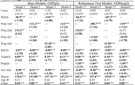
5.2.1 Results from Propositions 1 to 4
As shown in table 4, while the first main column of the table illustrates base-models
from equation (1) in the finance-growth nexus, the second shows corresponding robustness
checks of said models from equation (2) in the finance-welfare nexus. For instance “Model 1”
is checked by “Model 1*” and so forth. At first glance, regardless of estimated
coefficient-signs all propositions are independent significant determinants of growth and welfare. While
liquid liabilities and the informal financial sector reflect a negative finance-le-growth nexus,
the semi-formal financial sector accounts for the contrary. Semi-formal finance further weighs
heavily in the determination of the estimated coefficient sign of Proposition 4(when its effect
is combined with that of informal finance) .
Our controls for inflation, trade, government-expenditure and population growth are
significant with expected signs and consistent with recent empirical literature (Hassan et al.,
2011). Due to issues of multicolinearity and overparametization (see appendix 1) we could
Table 4: Regressions with propositions 1 to 4
Base Models: GDPg(l) Robustness Test Models: GDPpcg(l)
Model 1 Model 2 Model 3 Model 4 Model 1* Model 2* Model 3* Model4* Const. -0.53 -0.42 -1.32 -0.42 -0.16 -0.09 -0.87 -0.05
(-0.31) (-0.23) (-0.78) (-0.23) (-0.07) (-0.03) (-0.37) (-0.02) M2(d) -86.9*** --- -110*** --- -84.5*** --- -107.5***
---(-7.39) (-6.80) (-7.32) (-6.79)
Prop.1(d) --- -111.2*** --- -112*** --- -108.7*** --- -110***
(-7.33) (-7.23) (-7.32) (-7.21)
Prop.2(d) 115.2** --- --- 18.21 110.8** --- --- 16.73
(2.62) (0.47) (2.58) (0.44)
Prop.3(l) --- -11.52* --- -11.43* --- -11.04* --- -10.95*
(-1.84) (-1.82) (-1.80) (-1.78)
Prop.4(d) --- --- 93.38*** --- --- 91.89***
(3.05) (3.07)
Infl.(l) -0.07*** -0.09*** -0.09*** -0.09*** -0.07** -0.09*** -0.09*** -0.09***
(-2.39) (-3.28) (-3.07) (-3.30) (-2.35) (-3.23) (-3.03) (-3.25)
Trade(l) 0.09*** 0.11*** 0.10*** 0.11*** 0.08*** 0.10*** 0.10*** 0.10***
(3.22) (3.89) (3.77) (3.90) (2.99) (3.65) (3.53) (3.65)
Popg(l) --- --- --- --- -1.05** -1.04** -1.07** -1.05**
(-2.21) (-2.24) (-2.27) (-2.25)
Gov’t(d) -0.50*** -0.51*** -0.50*** -0.51*** -0.49*** -0.50*** -0.49*** -0.50***
(-4.25) (-4.41) (-4.26) (-4.41) (-4.24) (-4.40) (-4.26) (-4.41)
Hetero 178.6*** 157.08*** 157.74*** 147.21*** 183.1*** 157.8*** 159.8*** 148.6***
Adj. R² 0.33 0.36 0.34 0.35 0.36 0.39 0.37 0.38
Fisher 8.04*** 9.08*** 8.32*** 8.41*** 8.52*** 9.54*** 8.84*** 8.88*** (l): level. (d): first difference. *, **, ***: denote significance levels of 10%, 5% and 1% respectively. Prop: propositions. GDPpcg: GDP per capita growth. GDPg: GDP growth. LL (M2): Liquid Liabilities on GDP. Infl: Inflation. Popg: Population growth. Gov’t: Government expenditure. Hetero: Wald Chi-Square statistics for heteroscedasticity. Adj. R²: Adjusted Coefficient of determination. Fisher: Fisher statistics. Prop.1: formal financial sector development. Prop.2: semi-formal financial sector development. Prop.3: informal financial sector development. Prop.4: semi-formal and informal financial sectors development.
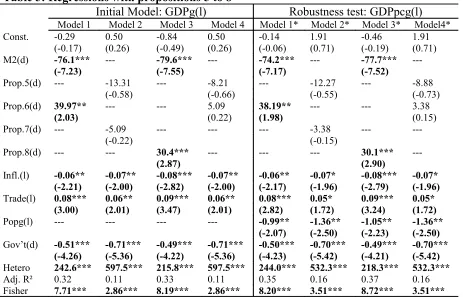
5.2.2 Results from Propositions 5 to 8
Regressions on indicators of sector importance presented in table 5 below have the
same structure as those of table 4 above. Our controls for inflation, trade,
government-expenditure and population growth are significant with expected signs and compatible with
recent empirical literature (Hassan et al., 2011). While propositions 6 and 8 are significant
with the right signs (as those of propositions 2 and 4 respectively in table 4), propositions 5
and 7 respectively for formal and informal finance sector importance are insignificant with the
right signs (as for propositions 1 and 3 respectively in table 4). Since propositions 5 and 7 are
not independently significant in the finance-growth nexus, we are poised to further verify
Table 5: Regressions with propositions 5 to 8
Initial Model: GDPg(l) Robustness test: GDPpcg(l)
Model 1 Model 2 Model 3 Model 4 Model 1* Model 2* Model 3* Model4* Const. -0.29 0.50 -0.84 0.50 -0.14 1.91 -0.46 1.91
(-0.17) (0.26) (-0.49) (0.26) (-0.06) (0.71) (-0.19) (0.71) M2(d) -76.1*** --- -79.6*** --- -74.2*** --- -77.7***
---(-7.23) (-7.55) (-7.17) (-7.52)
Prop.5(d) --- -13.31 --- -8.21 --- -12.27 --- -8.88
(-0.58) (-0.66) (-0.55) (-0.73)
Prop.6(d) 39.97** --- --- 5.09 38.19** --- --- 3.38
(2.03) (0.22) (1.98) (0.15)
Prop.7(d) --- -5.09 --- --- --- -3.38 ---
---(-0.22) (-0.15)
Prop.8(d) --- --- 30.4*** --- --- --- 30.1***
---(2.87) (2.90)
Infl.(l) -0.06** -0.07** -0.08*** -0.07** -0.06** -0.07* -0.08*** -0.07*
(-2.21) (-2.00) (-2.82) (-2.00) (-2.17) (-1.96) (-2.79) (-1.96)
Trade(l) 0.08*** 0.06** 0.09*** 0.06** 0.08*** 0.05* 0.09*** 0.05*
(3.00) (2.01) (3.47) (2.01) (2.82) (1.72) (3.24) (1.72)
Popg(l) --- --- --- --- -0.99** -1.36** -1.05** -1.36**
(-2.07) (-2.50) (-2.23) (-2.50)
Gov’t(d) -0.51*** -0.71*** -0.49*** -0.71*** -0.50*** -0.70*** -0.49*** -0.70***
(-4.26) (-5.36) (-4.22) (-5.36) (-4.23) (-5.42) (-4.21) (-5.42)
Hetero 242.6*** 597.5*** 215.8*** 597.5*** 244.0*** 532.3*** 218.3*** 532.3***
Adj. R² 0.32 0.11 0.33 0.11 0.35 0.16 0.37 0.16
Fisher 7.71*** 2.86*** 8.19*** 2.86*** 8.20*** 3.51*** 8.72*** 3.51*** (l): level. (d): first difference. *, **, ***: denote significance levels of 10%, 5% and 1% respectively. Prop: propositions. GDPpcg: GDP per capita growth. GDPg: GDP growth. LL (M2): Liquid Liabilities on GDP. Infl: Inflation. Popg: Population growth. Gov’t: Government expenditure. Hetero: Wald Chi-Square statistics for heteroscedasticity. Adj. R²: Adjusted Coefficient of determination. Fisher: Fisher statistics. Prop.5: formal financial sector development. Prop.6: semi-formal financial sector development. Prop.7: informal financial sector development. Prop.8: semi-formal and informal financial sectors development.
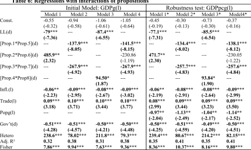
5.2.3 Results from interaction of propositions
Table 6 below covers regressions for the validity of hypothesis 4. As in the last two
tables, our controls for inflation, trade, government-expenditure and population growth are
significant with expected signs and consistent with recent empirical literature (Hassan et al.,
2011). The significance of interactions of propositions 1 and 5 on the one hand, and
propositions 3 and 7 on the other indirectly validate propositions 5 and 7. This implies that
though propositions 5 and 7 are not independent significant determinants of growth (table 5),
their interactions with propositions 1 and 3 are favorable to the finance-growth nexus.
Therefore with respect to our database, propositions 5 and 7 are valid if and only if there are
simultaneous improvements in proportions of GDP and shares in M2 for the formal and
informal financial sectors. Beyond this fact, our indirect validation of propositions 5 and 7
affect growth and welfare much higher than their independent effects combined. This also
[image:24.595.48.550.132.433.2]applies to semi-formal and informal sectors.
Table 6: Regressions with interactions of propositions
Initial Model: GDPg(l) Robustness test: GDPpcg(l)
Model 1 Model 2 Model 3 Model 4 Model 1* Model 2* Model 3* Model4* Const. -0.55 -0.94 -1.06 -1.05 -0.45 -0.30 -0.73 -0.37
(-0.32) (-0.58) (-0.61) (-0.64) (-0.19) (-0.13) (-0.30) (-0.16) LL(d) -79*** --- -87.4*** --- -77.1*** --- -85.5***
---(-7.36) (-6.55) (-7.31) (-6.54)
[Prop.1*Prop.5](d) --- -137.9*** --- -141.5*** --- -134.4*** --- -138.1***
(-8.05) (-8.15) (-8.02) (-8.12)
[Prop.2*Prop.6](d) 485.9** --- --- -230.86 471.7** --- --- -230.05
(2.32) (-1.19) (2.30) (-1.22)
[Prop.3*Prop.7](d) --- -267.9*** --- -267.9*** --- -257.7*** --- -257.6***
(-4.92) (-4.93) (-4.83) (-4.84)
[Prop.4*Prop8](d) --- --- 94.50* --- --- --- 93.84*
---(1.87) (1.90)
Infl.(l) -0.06** -0.09*** -0.08*** -0.09*** -0.06** -0.08*** -0.08*** -0.09***
(-2.23) (-2.95) (-2.67) (-3.02) (-2.19) (-2.91) (-2.64) (-2.99)
Trade(l) 0.09*** 0.10*** 0.10*** 0.10*** 0.08*** 0.09*** 0.09*** 0.09***
(3.18) (3.71) (3.44) (3.77) (2.99) (3.44) (3.23) (3.50)
Popg(l) --- --- --- --- -0.97** -1.13** -1.04** -1.14**
(-2.04) (-2.49) (-2.17) (-2.52)
Gov’t(d) -0.51*** -0.51*** -0.50*** -0.50*** -0.50*** -0.51*** -0.49*** -0.50***
(-4.28) (-4.57) (-4.21) (-4.48) (-4.25) (-4.59) (-4.20) (-4.51)
Hetero 238.6*** 78.02*** 211.8*** 79.3*** 239.4*** 80.67*** 214.2*** 82.15***
Adj. R² 0.32 0.38 0.31 0.38 0.35 0.41 0.35 0.41
Fisher 7.86*** 9.94*** 7.63*** 9.36*** 8.36*** 10.37*** 8.16*** 9.80*** (l): level. (d): first difference. *, **, ***: denote significance levels of 10%, 5% and 1% respectively. Prop: propositions. GDPpcg: GDP per capita growth. GDPg: GDP growth. LL (M2): Liquid Liabilities on GDP. Infl: Inflation. Popg: Population growth. Gov’t: Government expenditure. Hetero: Wald Chi-Square statistics for heteroscedasticity. Adj. R²: Adjusted Coefficient of determination. Fisher: Fisher statistics. [Prop.1*Prop.5]: formal financial sector development. [Prop.2*Prop.6]: semi-formal financial sector development. [Prop.3*Prop.7]: informal financial sector development. [Prop.4*Prop.8]: semi-formal and informal financial sectors development.
For tables 4, 5 and 6, the Fisher and Wald statistics for respectively the significance of
overall model and justification of the use of GLS are significant for all regressions.
Explanatory powers of estimated parameters expressed by the adjusted coefficient of
determination (Adj.R²) are also impressive.
5.2.4 Retrospect to hypotheses
Hypothesis 1: “The informal financial sector (a previously missing component in the
definition of monetary base: M2) significantly contributes to economic growth”.
We have verified the empirical validity of propositions 3 and 7 resulting from this
finance-growth nexus, simultaneous improvements of propositions 3 and 7 indirectly validate
Proposition 7 by virtue of hypothesis 4.
Hypothesis 2: “Disentangling different components of the existing measurement (financial
system) into formal (banking sector) and semi-formal (other financial institutions) financial
sector indicators could improve understanding of the finance-growth nexus”.
We have equally verified this hypothesis. While in tables 4, 5 and 6, coefficients of
M2 have been significantly negative, those corresponding to formal and semi-formal finance
have been negative and positive respectively. This suggests formal finance is the more
important determinant of M223. However disentangling the semi-formal finance sector yields a
different significant sign (positive) in the finance-growth nexus. This implies had M2 been
used as the sole financial indicator, its negative sign (geared by formal finance) would have
over-shadowed the positive sign of semi-formal finance contained there-in. Consequently
disentanglement has improved our understanding of the finance-growth nexus.
Hypothesis 3: “Introducing measures of sector importance could ameliorate the capacity to
understand how evolvements (improvements) of shares in different sectors of the financial
system affect the finance-growth nexus”.
But for the semi-formal financial sector in which a great part of information in
Proposition 2 in reflected in Proposition 6(approximately 90%), only 51% and 23% of
information in propositions 1 and 3 are present in propositions 5 and 7 respectively(see
correlation analysis in appendix). This suggests that sector importance finance indicators are
not the same as GDP ratio indicators (: they are complements to GDP ratio measures). Thus,
though the finance-led-growth effects of similar sectors in the two categories of indicator
(GDP or M2 ratios) have the same sign and significance, our data structure by virtue of
23
correlation analysis shows same sector M2 ratios and sector GDP ratios are not the same(: do
not contain the same information ). Vertically comparing coefficients from regressions in
tables 4, 5 and 6, it could be deduced that the finance growth-nexus is more affected by
proportion-of-GDP financial-sector ratios than shares-of-M2 ratios(: further evidence that the
two sets of indicators contain information with different variations).
Hypothesis 4: “For formal finance, simultaneous improvement in shares of GDP (Prop.1)
and Monetary Base (Prop.5) should have a higher impact on Growth (than their combined
independent effects). By the same token, this applies to semi-formal finance (Prop.2 and
Prop.6) and informal finance (Prop.3 and Prop.7)”.
We have shown that, though sector GDP ratios or sector M2 ratios are independent
significant determinants of growth, simultaneous improvements in sector shares of GDP and
M2 will yield a greater effect on growth than their combined independent effects. Thus policy
oriented towards simultaneously increase of shares in both categories of ratios should yield
higher growth-effects.
6. Conclusion
Financial development indicators are often applied to countries/regions without taking
into account specific financial development realities. Financial depth in the perspective of
monetary base is not equal to liquid liabilities in every development context. This paper has
introduced complementary indicators to the existing Financial Development and Structure
Database (FDSD).
We have empirical tested four hypotheses and withheld the following: (1) the informal
financial sector (a previously missing component in the definition of the monetary) base)
existing measurement (financial system) into formal (banking sector) and semi-formal (other
financial institutions) financial sector indicators improves understanding of the
finance-growth nexus; (3) introducing measures of sector importance could ameliorate the capacity to
understand how evolvements (improvements) of shares in different sectors of the financial
system affect the finance-growth nexus; (4) though sector GDP ratios or sector M2 ratios are
independent significant determinants of growth, simultaneous improvements in sector shares
of GDP and M2 will yield a greater effect on growth than their combined independent effects.
The work unites two streams of research. It contributes at the same time to the
macroeconomic literature on measuring financial development and responds to the growing
field of economic development by means of informal financial sector promotion and
microfinance. The paper suggests a practicable way to disentangle the effects of the various
Appendices
Appendix 1 : Correlation analysis
LL Prop1 Prop2 Prop3 Prop4 Prop5 Prop6 Prop7 Prop8 Infl. Trade GDPg GDPpc Popg Gov 1.00 0.97 0.27 0.76 0.74 0.33 0.04 -0.39 -0.33 -0.21 0.29 -0.04 0.08 -0.57 0.04 LL
1.00 0.12 0.44 0.42 0.51 -0.08 -0.47 -0.51 -0.23 0.38 -0.02 0.11 -0.63 0.05 Prop1 1.00 0.13 0.53 -0.40 0.90 -0.34 0.40 0.16 -0.02 -0.08 -0.09 0.04 0.03 Prop2 1.00 0.90 -0.12 -0.12 0.23 0.12 -0.27 -0.00 -0.16 -0.10 -0.23 0.03 Prop3 1.00 -0.32 0.41 -0.01 0.32 -0.16 -0.01 -0.17 -0.13 -0.17 0.04 Prop4 1.00 -0.47 -0.65 -1.00 -0.20 0.54 0.00 0.09 -0.45 -0.02 Prop5 1.00 -0.35 0.47 0.30 -0.05 -0.04 -0.08 0.16 0.00 Prop6 1.00 0.65 -0.04 -0.53 0.03 -0.02 0.33 0.02 Prop7 1.00 0.20 -0.54 -0.00 -0.09 0.45 0.02 Prop8 1.00 0.01 0.00 -0.02 0.16 0.01 Infl.
1.00 -0.06 0.02 -0.43 -0.01 Trade 1.00 0.98 -0.04 -0.10 GDPg 1.00 -0.23 -0.08 GDPpc
References
Abu-Bader, S., & Abu-Qarn, A.S., 2008. “Financial Development and Economic Growth:
Empirical Evidence from Six MENA countries”, Review of Development Economics, 12(4),
pp. 803-817.
Ang, J.B. & McKibbin, W.J., 2007. “Financial Liberalization, financial sector development
and growth: Evidence from Malaysia”, Journal of Development Economics, 84, pp.215-233.
Asongu, S. A., 2010a. “Stock market development in Africa: do all macroeconomic financial
intermediary determinants matter?” MPRA Paper 26910.
Asongu, S. A., 2010b. “Bank efficiency and openness in Africa: do income levels matter?”
MPRA 27025.
Asongu, S. A., 2011. “How would population growth affect investment in the future?
Asymmetric penal causality evidence for Africa”, MPRA Paper 30124.
Aryeetey, E., 2008, March. “From Informal Finance to Formal Finance in Sub-Saharan
Africa: Lessons from Linkage Efforts”, Institute of Statistical, Social and Economic
Research, University of Ghana.
Claessens, Stijn, Demirgüç-Kunt, A, & Huizinga, H., 2001. “How does foreign entry affect
the domestic banking market? Journal of Banking and Finance 25 (May), pp. 891–911.
Demetriades, P.O., & Hussein, K.A., 1996. “Does Financial Development Cause Economic
Growth? Time-Series Evidence from Sixteen Countries,” Journal of Development Economics,
51, pp.387-411.
Demirguc-Kunt, A., Beck, T., & Levine, R., 1999. “A New Database on Financial
Development and Structure”, International Monetary Fund, WP 2146.
Demirguc-Kunt, A., & Beck, T., 2009, May. “Financial Institutions and Markets Across
Countries over time: Data and Analysis”, World Bank Policy Research Working Paper No.
Gries, T., Kraft, M., & Meierrieks, D., 2009. “Linkages between financial deepening, trade
openness, and economic development: causality evidence from Sub-Saharan Africa”, World
Development, 37(12), pp. 1849-1860.
Hassan, K., Sanchez, B., & Yu, J., 2011. “Financial development and economic growth: New
evidence from panel data”, The Quarterly Review of Economics and Finance, 51, pp.88-104.
Im, K.S., Pesaran, M.H., & Shin, Y., 2003. “Testing for unit roots in heterogeneous panels”,
Journal of Econometrics", 115, pp.53-74.
IMF Statistics Department, 2008, October. “International Financial Statistics Yearbook,
2008”, IMF
Kablan, S., 2010. “Banking Efficiency and Financial Development in Sub-Saharan Africa”,
IMF Working Paper /10/136
Khim, V. L. S., 2004. “Which lag selection criteria should we employ”, Economics Bulletin,
3(33), pp.1-9.
King, R.G., & Ross, L., 1993. “Finance and Growth: Schumpeter Might Be Right”, Quarterly
Journal of Economics, 108, pp. 717-737.
Kumbhakar, S.C. and Mavrotas, G., 2005. “Financial Sector Development and Productivity
Growth”. UNUWIDER Research Paper: 2005/68, World Institute for Development
Economics Research at the United Nations University.
Levin, A., Lin, C.F., & Chu, C.S., 2002. “Unit root tests in panel data: asymptotic and
finite-sample properties”, Journal of Econometrics, 108, pp. 1-24.
Levine, R., & King, R.G., 1993. “Finance and Growth: Schumpeter Might be Right”, The
Quarterly Journal of Economics, 108, pp.717-737.
Maddala, G.S., & Wu, S., 1999. “A Comparative Study of Unit Root test with Panel Data and
Steel, W.F., 2006. “Extending Financial Systems to the poor: What strategies for
Ghana”,Paper presented at the 7th ISSER-Merchant Bank Annual Economic Lectures,
University of Ghana, Legon.