A Perturbative Based Generalized Series Expansion in Terms of Non Orthogonal Component Functions

(1)

http://www.scirp.org/journal/am ISSN Online: 2152-7393

ISSN Print: 2152-7385

A Perturbative-Based Generalized Series

Expansion in Terms of Non-Orthogonal

Component Functions

Robert B. Szlavik1, Dana Paquin2, Galen E. Turner III3

1_{Department of Biomedical Engineering, California Polytechnic State University, San Luis Obispo, USA} 2_{Department of Mathematics, California Polytechnic State University, San Luis Obispo, USA}

3_{Department of Mathematics and Statistics, Louisiana Tech University, Ruston, USA}

Abstract

In this paper we present a generalized perturbative approximate series expan-sion in terms of non-orthogonal component functions. The expanexpan-sion is based on a perturbative formulation where, in the non-orthogonal case, the contribution of a given component function, at each point, in the time do-main or frequency in the Fourier dodo-main, is assumed to be perturbed by con-tributions from the other component functions in the set. In the case of or-thogonal basis functions, the formulation reduces to the non-perturbative case approximate series expansion. Application of the series expansion is demon-strated in the context of two non-orthogonal component function sets. The technique is applied to a series of non-orthogonalized Bessel functions of the first kind that are used to construct a compound function for which the coef-ficients are determined utilizing the proposed approach. In a second applica-tion, the technique is applied to an example associated with the inverse prob-lem in electrophysiology and is demonstrated through decomposition of a compound evoked potential from a peripheral nerve trunk in terms of con-tributing evoked potentials from individual nerve fibers of varying diameter. An additional application of the perturbative approximation is illustrated in the context of a trigonometric Fourier series representation of a continuous time signal where the technique is used to compute an approximation of the Fourier series coefficients. From these examples, it will be demonstrated that in the case of non-orthogonal component functions, the technique performs significantly better than the generalized Fourier series which can yield non-sensical results.

Keywords

Non-Orthogonal Functions, Series Expansion, Approximate Series Expansion, Perturbative-Based Approximate Expansion, Numerical Approximations

How to cite this paper: Szlavik, R.B., Pa-quin, D. and Turner III, G.E. (2017) A Perturbative-Based Generalized Series Ex-pansion in Terms of Non-Orthogonal Com- ponent Functions. Applied Mathematics, 8, 106-116.

http://dx.doi.org/10.4236/am.2017.81009

Received: October 26, 2016 Accepted: January 22, 2017 Published: January 25, 2017

http://creativecommons.org/licenses/by/4.0/

(2)

1. Introduction

We propose the following novel approximate generalized series expansion for a function ψ

( )

t in terms of a finite number of component functions

{

( )

}

1

m

n t _n

λ ₌

where the component functions do not necessarily satisfy the orthogonality condition or form a basis for the function space:

( )

1 . m n n n

t t t

ψ ψ β λ

=

∼  =

∑

 (1)

Let ψ

( )

t :

[ ]

a b, → be a square-integrable function and let

( )

f ψ

( )

t

Ψ =_ _ (2)

be the Fourier transform of ψ

( )

t .

In the expansion proposed in Equation (1), the component functions λn

( )

t

may be orthogonal or non-orthogonal. In the event that there is an infinite number of component functions that are orthogonal, satisfying the condition that any λa

( )

t and λb

( )

t , on the interval τ1≤ ≤t τ2 are such that

( ) ( )

2 1

d 0

a t b t t τ

τ λ λ =

∫

, the expansion is exactly yielding an equality in the expre-

ssion shown in Equation (1). For a finite set of non-orthogonal component functions, the expansion is approximate.

The coefficients βn may be determined using a perturbative approach where

it is assumed that, at any given value of t, the contribution of each component

function λn

( )

t to the function ψ

( )

t is perturbed by contributions from the

other component functions in the set. From the perspective of the Fourier domain, it may be said that each frequency component of Ψ

( )

f consists of

contributions from the corresponding frequency component of each component function Λn

( )

f where

( )

n f λn t

Λ =_ _ (3)

is the Fourier transform of the th

n component function λn

( )

t .

The above description associated with a perturbed contribution of each of the component functions Λn

( )

f to the corresponding frequency components of

( )

f

Ψ can be written mathematically as shown in Equation (4). The

coefficients i j, are the variables associated with the relative magnitude of the

perturbative contribution of the other component functions to the frequency component of the component function Λn

( )

f .

( )

1 2,1 1 ,1 1

1,2 2 2 ,2 2

1, 2,

m

m m m m m

f f f

f

f f f

Λ Λ Λ

+ + +

Λ Λ Λ

+ +

Ψ = + + + +

+ + +

Λ Λ Λ

          (4)

(3)

( )

2,1 ,1 1,2 ,2 1 2 1, 2, 1 1 1 1 1 1 m m m m m

f f f f

   

   

Ψ = Λ_ Λ Λ _{ } _{  }

             _ _ _         (5)

Evaluating Equation (4) or Equation (5) at a specific frequency fk for

1

k= l and re-arranging so as to isolate the terms with the variables i j, on

the right hand side yields Equation (6).

( )

,

( )

1 1 1

m m

m

k i k i j j k

i j i

i j

f f f

= = =

≠

Ψ − Λ

∑

=

∑∑

 Λ (6)

The system of equations described by Equation (6) is such that 2

l>m −m

which constitutes an over-determined linear system. The value of l is the

chosen number of frequency points at which (6) is evaluated. It is then possible to solve the linear equations, in the least squares sense, for the complex values of the variables i j, .

Using the decomposition in Equation (4), we define the following superposition of each component function Λn,n=1m to be BnΛn:

( )

1, 1,

1, , .

n n n n n n n

n n n n m n n

B f f f

f f f

−

+

Λ = Λ + + Λ

+ Λ + Λ + + Λ

 _



 

  (7)

The complex estimator Bn, 1, 2,∀ =n ,m is defined as:

1, 1, 1 1, , .

n n n n n n m n

B = + + ₋ + +₊ + +  (8)

Since Bn is complex, its magnitude Bn will yield the multiplicative

coefficient βn by which each component function must be scaled as per

Equation (1)

,

n Bn B Bn n

β ₌ _ ₌ _{ }∗ ₍₉₎

where Bn ∗

 _{is the complex conjugate of} B_n.

2. Examples

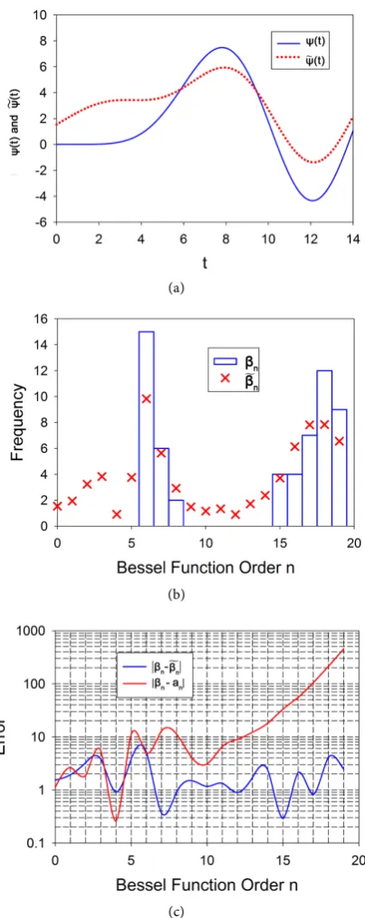
2.1. Example 1. Bessel Functions

In this first example, we utilize the proposed series expansion to estimate the coefficients associated with the sum of non-orthogonal Bessel functions Jn

( )

t

of the first kind, where n is a positive integer, as described in Equation (10)

[1]:

( )

₍

₎

2 0

1

. ! ! 2

z z n

n z

t J t

z z n

+ ∞ = −   = _{ } +  

∑

(10)

A compound function was generated through the superposition of a series of Bessel functions of the first kind with a set of coefficients as per Equation (11):

( )

6 7 8 15

16 17 18 19

15 6 2 4

4 7 12 9 .

t J t J t J t J t

J t J t J t J t

ψ = + + +

(4)

Figure 1 illustrates the results of the proposed series expansion for determining the coefficients of a series of superposed non-orthogonal Bessel functions. A comparison is shown in a) of the template compound function ψ

( )

t with the

estimated compound function ψ

( )

t generated using the estimated coefficients

n

β _{. The graph in b) is a comparison of the actual distribution coefficient values}

n

β _{, shown in the histogram, with the estimated distribution coefficient values}

n

β _{. A graph of the error magnitude is given in c) between the actual distribution}

coefficients and the estimated coefficient values βn−βn as well as the error magnitude between the actual distribution coefficients and the generalized Fourier series coefficients β −n an . The generalized Fourier series coefficients

n

a are found from Equation (12)

( )

2 ₀

( ) ( )

1

d

f

n n

n

a t t t

t

τ ψ

= Λ

Λ

∫

(12)

where

( )

2

( ) ( )

0 d

f

n t n t n t t

τ

Λ =

_∫

Λ Λ [2].

2.2. Example 2. The Inverse Problem in Electrophysiology

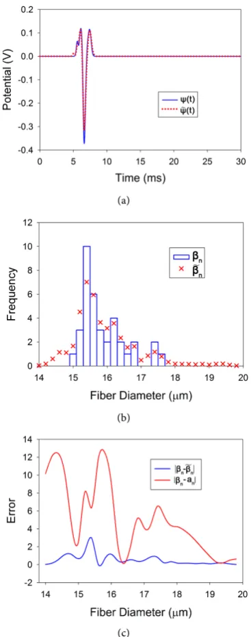
The inverse problem in electrophysiology involves utilization of recorded biopotentials to determine the characteristics of the biological signal generator that gives rise to the recorded biopotential signals. A specific situation, in the context of the inverse problem, arises when it is necessary to determine the conduction velocity or size distribution of a population of peripheral nerve fibers from a recorded compound evoked potential. The compound evoked potential, to a first approximation, may be viewed as the superposition of the single fiber evoked potentials associated with the individual nerve fibers in the nerve trunk that have been electrically activated. Information related to the size distribution, which is linearly related to the conduction velocity distribution of nerve fibers in the evoked population, is of clinical use because different disease processes selectively impact different segments of the nerve population having different diameter or size [3] [4].

When the separation of nerve fiber sizes is relatively large, the resultant single fiber evoked potentials are orthogonal to each other and a generalized Fourier series may be used to estimate the size distribution. In the event that the fiber size classes are such that there is significant temporal overlap between their associated single fiber evoked potentials, the generalized Fourier series can yield nonsensical results. In such cases, the perturbative decomposition outlined in this paper may be used to obtain an estimate of the coefficients associated with the series expansion shown in Equation (1) as first demonstrated by Szlavik [5].

(

)

(

)

{

2 2 2 2 2 2

}

,

exp exp 1 exp

y vy t y r

λ δ

α α

 ⋅ − 

 

     

= Φ _−Γ ϒ −_ _−Γ Ξ + −_ _−Γ Θ _ (13)

where

2

4π

y e y

D

a σ

(5)

(a)

(b)

[image:5.595.275.477.68.576.2]

(c)

Figure 1. Graphs illustrating the results of the proposed series expansion for determining the coefficients of a series of superposed non-orthogonal Bessel functions. A comparison is shown in (a) of the template compound function ψ

( )

t with the estimated compound

function ψ

( )

t generated using the estimated coefficients β_n. The graph in (b) is a

comparison of the actual distribution coefficient values βn, shown in the histogram,

with the estimated distribution coefficient values βn. A graph of the error magnitude is

given in (c) between the actual distribution coefficients and the estimated coefficient values β βn− n as well as the error magnitude between the actual distribution coeffi-

cients and the generalized Fourier series coefficients βn−an . The generalized Fourier

(6)

4 y D

Γ = (15)

(

)

y y y

y

v t s

a

δ

⋅ − +

ϒ = ₍₁₆₎

(

)

y y y

y

v t s

a

δ

⋅ − −

Ξ = ₍₁₇₎

(

)

y y y

y

v t u

a

δ

⋅ − −

Θ = ₍₁₈₎

To illustrate the applicability of the perturbative expansion to the case where the single fiber evoked potentials are non-orthogonal, we generated a population of one hundred nerve fibers, using the distribution shown in Equation (19), with

diameters ranging from 16 μm to 20 μm using a technique outlined by

[image:6.595.340.540.75.215.2]

Szlavik et al. [6]. The population was generated with the parameters shown in

Table 1 which were established from an empirical study [7].

( )

4

(

)

2

2 1 exp 2 2π y h h d y

h h h

d

p d σ µ

γ γ =  ₋    = −    

∑

(19)

Each fiber y in the population of z fibers was then sorted into one of the fiber size classes n, for n=130, having a separation in diameter of 0.2 μm

where the single fiber evoked potentials, shown in Equations (13) through (18), associated with the th

n size classes are not orthogonal and are generated using the

function proposed by Fleisher et al. in Equation (6) of their paper [8]. All parameters in Equations (13) through (18) are as described in Fleisher and were assigned values

2 y y

a =d , sy= ⋅1 ay , r =1 mm , vy = ⋅c dy , α =0.998 , σ =e 1.0 S m ,

Table 1. Parameter values used in the fiber diameter distribution shown in Equation (19).

[image:6.595.210.539.500.736.2]

(7)

(

) (

)

y y y y

D = a +s r+s , uy=sy

(

1+α

) (

1−α

)

, δ =y x vy where dy is the

fiber diameter and x is the propagation distance. The function has been

normalized to the current through the second pole such that λ =y g I where 1 A

I = .

An activation function ξ

( )

dy was used to determine what stimulus current amplitude was sufficient to excite each fiber with diamater dy as per Equation

(20) where ζ =10 mA and η=3.5 10 m× 5 −1.

( )

d_y exp d_y

ξ =ζ _−η _₍₂₀₎

The time domain representation of the compound evoked potential ψ

( )

t

may be written as a summation over z fibers in the population, as per

Equation (21), where the contribution of a given single fiber evoked potential of a given class n y

( )

associated with the th

y fiber is only added in when the

stimulus current amplitude Ω is greater than the activation current for the given fiber diameter as quantified in Equation (20) [9].

( )

( ) ( )

(

( )

)

1

,

z

y n y n y n y

y

t u d v t r

ψ ξ λ δ

=

 

=

∑

_Ω − _ _ ⋅ − _₍₂₁₎

Figure 2 illustrates the results of the proposed series expansion for estimating the diameter distribution of the nerve fibers contributing to the compound evoked potential for the population generated as described earlier. A comparison is shown in a) of the template compound evoked potential ψ

( )

t with the

estimated compound evoked potential ψ

( )

t generated using the estimated

coefficients βn. The graph in b) is a comparison of the actual fiber diameter

distribution coefficient values βn, shown in the histogram, with the estimated

fiber diameter distribution coefficient values βn. A graph of the error magni-

tude is given in c) between the actual distribution coefficients and the estimated coefficient values βn−βn as well as the error magnitude between the actual distribution coefficients and the generalized Fourier series coefficients β −n an

where the coefficients an are found using Equation (12).

2.3. Example 3. Continous Time Signals

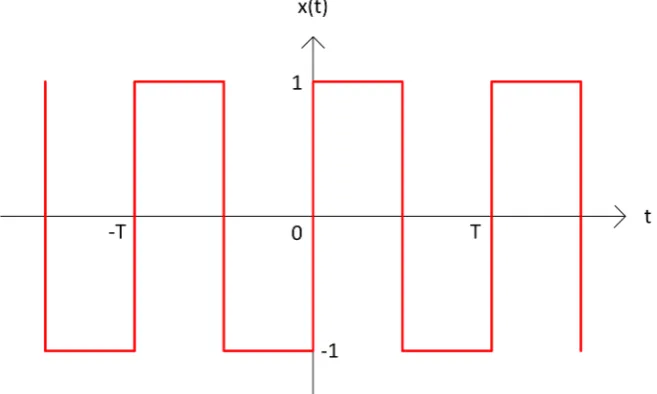
In the theory of continuous time signals, a periodic square waveform with a periodicity of T , a fundamental frequency of fo =1T or ω =o 2πfo in

radians per second may be represented using a trigonometric Fourier series expansion as per (22) [10]:

( )

(

)

(

)

1

cos sin .

o n o n o

n

x t a α nωt β nω t

∞

=

 

= +

∑

_ + _ ₍₂₂₎

For a square waveform of the type shown in Figure 3, the average value of the waveform is zero yielding a coefficient a0=0. The waveform may be appro-

ximated as a superposition of an infinite series of sinusoidal waveforms and thus the coefficients of the cosine term in the series expansion of (22) are α =n 0.

Evaluation of the Fourier coefficients for the sinuosidal term in (22) yields

( )

4 π

n n

(8)

(a)

(b)

[image:8.595.282.466.68.534.2]

(c)

Figure 2. Graphs illustrating the results of the proposed series expansion for determining the diameter distribution of the nerve fibers contributing to a compound evoked potential. A comparison is shown in (a) of the template compound evoked potential ψ

( )

t with

the estimated compound evoked potential ψ

( )

t from the estimated coefficients β_n.

The graph in (b) is a comparison of the actual fiber diameter distribution coefficient values βn with the estimated fiber diameter distribution coefficient values βn. A graph

of the error is given in (c) between the actual distribution coefficients and the estimated coefficient values β βn−n as well as the error magnitude between the actual distribu-

tion coefficients and the generalized Fourier series coefficients βn−an where the

coefficients an are found using Equation (12). The parameters for the neural simulation

were α=0.998, σe=1 S m,

5 1

5 10 s

c= × − , where m=30 is the number of diameter classes, Ω =50 μA is the stimulus current amplitude, x=0.05 m is the propagation

distance and 3

1.74 10

(9)

[image:9.595.209.538.75.272.2]

Figure 3. Square wave with fifty percent duty cycle and zero volt DC offset.

An approximation to (22) may be obtained if we limit the number of terms in the series expansion to a finite value as in (23):

( )

(

)

1

sin .

m

n o

n

x t x t β nω t

=

∼ =

∑

 (23)

If we apply the perturbative approach, the sinusoidal functions in (23) may be considered to form the component functions λn

( )

t . The coefficient estimates

n

β _{may be determined using the technique proposed herein.}

Figure 4 illustrates application of the perturbative approach to a square waveform of the type shown in Figure 3 for an approximate series consisting of

20

m= terms and a fundamental frequency fo =1 10π

( )

. A comparison is

shown in a) of the template square waveform estimate ψ

( )

t with the approxi-

mated waveform ψ

( )

t from the estimated Fourier coefficients βn. The graph

in b) is a comparison of the actual Fourier series coefficient values βn with the

estimated coefficient values βn. A graph of the error is given in c) between the

Fourier series coefficients and the estimated coefficient values βn−βn . The perturbative expansion provides a robust estimate of the Fourier series coefficients. The accuracy of the estimated coefficients is not unexpected since the component functions are orthogonal.

3. Conclusions

(10)

(a)

(b)

(c)

Figure 4. Graphs illustrating the results of the proposed perturbative expansion for determining estimates of the Fourier series coefficients. A comparison is shown in (a) of the template square waveform estimate ψ

( )

t with the approximated waveform ψ

( )

t

from the estimated Fourier coefficients βn. The graph in (b) is a comparison of the

actual Fourier series coefficient values βn with the estimated coefficient values βn. A

graph of the error is given in (c) between the Fourier series coefficients and the estimated coefficient values β βn−n . The parameters for the approximated square waveform were

20

[image:10.595.266.489.68.604.2]

(11)

ted to the inverse problem in electrophysiology presented in Szlavik [5], the accuracy of the estimated series coefficients degrades as the degree of temporal overlap, or non-orthogonality, of the component functions increases.

The technique would appear to have broad applicability in electrophysiology and the neurosciences particularly with respect to determination of the characteristics of signal generators as related to the inverse problem. Currently investi- gation of the decomposition of postsynaptic potentials into the contributions of constituent receptor-ligand complexes is being undertaken. The technique is general in the sense that it may be applied in situations where a compound function is known to consist of the superposition of orthogonal or non-orthogonal component functions which are also known.

References

[1] Lomen, D. and Mark, J. (1988) Differential Equations. Prentice-Hall, Englewood Cliffs.

[2] Kreyszig, E. (1988) Advanced Engineering Mathematics, Vol. 6. John Wiley & Sons, New York.

[3] Harati, Y. (1987) Diabetic Peripheral Neuropathies. Annals of Internal Medicine, 107, 546-559.https://doi.org/10.7326/0003-4819-107-4-546

[4] Dorfman, L., Cummins, K., Reaven, G., Ceranski, J., Greenfield, M. and Doberne, L. (1983) Studies of Diabetic Polyneuropathy Using Conduction-Velocity Distribution (dcv) Analysis. Neurology, 33, 773-779.https://doi.org/10.1212/WNL.33.6.773

[5] Szlavik, R. (2016) A Perturbation Based Decomposition of Compound Evoked Po-tentials for Characterization of Nerve Fiber Size Distributions. IEEE Transactions on Neural Systems and Rehabilitation Engineering, 24, 212-216.

https://doi.org/10.1109/TNSRE.2015.2476917

[6] Szlavik, R. and de Bruin, H. (1997) Simulating the Distribution of Axon Size in Nerves. CMBES/SCGB, 168-169.

[7] Boyd, I.A. and Davey, M.R. (1968) Composition of Peripheral Nerves. E. & S. Li-vingstone, Edinburgh.

[8] Fleisher, S., Studer, M. and Moschytz, G. (1984) Mathematical-Model of the Sin-gle-Fiber Action-Potential. Medical & Biological Engineering & Computing, 22, 433-439.https://doi.org/10.1007/BF02447703

[9] Szlavik, R. (2008) A Novel Method for Characterization of Peripheral Nerve Fiber Size Distributions by Group Delay. IEEE Transactions on Biomedical Engineering, 55, 2836-2840.https://doi.org/10.1109/TBME.2008.921149

(12)

Submit or recommend next manuscript to SCIRP and we will provide best service for you:

Accepting pre-submission inquiries through Email, Facebook, LinkedIn, Twitter, etc. A wide selection of journals (inclusive of 9 subjects, more than 200 journals)

Providing 24-hour high-quality service User-friendly online submission system Fair and swift peer-review system

Efficient typesetting and proofreading procedure

Display of the result of downloads and visits, as well as the number of cited articles Maximum dissemination of your research work

Submit your manuscript at: http://papersubmission.scirp.org/