Real Exchange Rates and Productivity: Evidence From Asia

(1)

Munich Personal RePEc Archive

Real Exchange Rates and Productivity:

Evidence From Asia

Yan, Isabel K. and Kakkar, Vikas

City University of Hong Kong

September 2011

Online at

https://mpra.ub.uni-muenchen.de/35218/

(2)

Real Exchange Rates and Productivity: Evidence From Asia

Vikas Kakkar and Isabel Yanyz

Department of Economics and Finance

City University of Hong Kong

Abstract This paper examines a productivity-based explanation of the long run

real exchange rate movements of six Asian economies. Using industry level data,

we construct total factor productivities (TFPs) for the tradable and nontradable

sectors. We …nd that (a) within each country the relative price of nontradable goods

is cointegrated with the sectoral TFP di¤erential, and (b) the real exchange rates

are cointegrated with the home and foreign sectoral TFP di¤erentials. Using the

predicted real exchange rate as a measure of the "long-run equilibrium", we …nd that

most Asian economies’ real exchange rates are overvalued before the Asian Financial

Crisis.

Keywords: Nontraded Goods, Balassa-Samuelson Model, Cointegration

JEL Classi…cation System: F31, F41

Corresponding author: Associate Professor, Department of Economics and Finance, City Univer-sity of Hong Kong, Kowloon Tong, Hong Kong, E-Mail: efvikas@cityu.edu.hk; Tel: +852-34429707; Fax: +852-34420284

y_{Assistant Professor, Department of Economics and Finance, City University of Hong Kong,}

Kowloon Tong, Hong Kong, E-Mail: efyan@cityu.edu.hk; Tel: +852-34427315; Fax: +852-34420284

z_{We would like to thank, without implicating, Yoosoon Chang, Yin-Wong Cheung, Menzie Chinn,}

(3)

1 Introduction

Of the several competing explanations for the persistent deviations of nominal

ex-change rates from their Purchasing Power Parities (PPPs), perhaps the earliest and

most fundamental is the productivity di¤erential hypothesis proposed by Balassa

(1964) and Samuelson (1964). The Balassa-Samuelson hypothesis (henceforth B-S)

asserts that di¤erent trends in tradable and nontradable sectors’ productivity cause

systematic departures of exchange rates from PPPs by changing the relative price

of nontradable (to tradable) goods.1 _{Since the B-S model relies on di¤erential}

pro-ductivity growth rates, we would expect it to be especially relevant for determining

the real exchange rates of the relatively fast growing Asian economies. However, the

relatively sparse literature on Asian real exchange rates o¤ers little support for the

key predictions of the B-S model.

Ito, Isard and Symansky (1999) document a positive correlation between growth

rates (relative to the U.S.) and real exchange rate appreciation for a group of East

Asian economies. However, they …nd that the relationship between the real exchange

rate and the relative price of nontradables seldom conforms to the B-S model. Chinn

(1996) …nds evidence of cointegration between relative prices of nontradables and

real exchange rates for selected Asian economies with some exceptions. A later study

by Chinn (2000) …nds evidence of a cointegrating relationship between real exchange

rates and labor productivity di¤erentials for only three out of the nine Asian countries

in his sample (Japan, Malaysia and the Philippines). Thomas and King (2008) extend

Chinn’s sample to include other Asian economies, but …nd similarly mixed evidence for

cointegration between real exchange rates and labor productivity di¤erentials despite

including a host of other variables in their regressions.

To our understanding, studies in the extant literature have focused solely on labor

1_{Obstfeld and Rogo¤ (1996, Chapter 4) provides an excellent overview of the theory and evidence}

(4)

productivity data since capital stock data for the Asian economies are generally not

available. An important limitation of using labor productivity data is that one is

unable to separate the impact of the supply-side e¤ects from demand-side e¤ects.2

The B-S model is quintessentially about the impact of di¤erent trends in

techno-logical progress in the traded and nontraded goods sectors on the relative price of

nontraded to traded goods and the real exchange rate.3 _{Therefore, a priori, there is}

a greater likelihood of uncovering a link between real exchange rates and di¤erential

technological trends, if one exists, by using a theoretically more appropriate measure

of technological progress.4

In this paper, we construct measures of sectoral total factor productivity (TFP)

for six Asian economies (Hong Kong, Indonesia, Korea, Malaysia, Singapore, and

Thailand) which are more consistent with the theory underlying the B-S model. We

…rst construct estimates of the aggregate capital stock of each Asian economy

us-ing investment data. The gross capital stock is then allocated to the tradable and

nontradable sectors in proportion to the share of capital income in that sector. The

TFPs for the tradable and nontradable sectors of these economies are then computed

as residuals from a Cobb-Douglas production function. The sectoral TFP data allows

us to gauge the economic signi…cance of the Balassa-Samuelson e¤ect for the bilateral

real exchange rates of these Asian countries against the U.S. dollar.

Given that most of the Asian countries in our sample had pegged their exchange

2_{For example, Drine and Rault (2002) do not …nd any evidence of cointegration between real}

exchange rates and labor productivity di¤erentials for six Asian economies using Pedroni’s (1999, 2004) panel cointegration tests. They attribute this failure to the fact that relative prices of non-tradables within each country are not cointegrated with the domestic sectoral labor productivity di¤erentials. Choudhri and Khan (2004), who use a larger panel of sixteen developing economies and similar panel cointegration methods as Drine and Rault (2002), uncover more favorable evidence for the B-S model.

3_{The real exchange rate is de…ned as the ratio of the domestic price level to the foreign price}

level multiplied by the nominal exchange rate. With this de…nition, deviations of nominal exchange rates from PPP are synonymous with changes in the real exchange rate.

4_{A similar point is made by De Gregorio, Giovannini and Krueger (1994) and Kakkar (2003) in}

(5)

rates to the U.S. dollar, it is also of interest to examine the implications of the

pro-ductivity based model for real exchange rate misalignment prior to the Asian …nancial

crisis. One noteworthy feature of this approach to measuring real exchange rate

mis-alignment is that, since the real exchange rate is cointegrated with the productivity

di¤erentials, any deviation between the actual real exchange rate and its estimated

equilibrium value is only temporary and will eventually vanish. This is a natural

requirement for any measure of an "equilibrium" value but is not satis…ed by the

oft-used PPP-based measures of misalignment. Alba and Papell (2007) test for the

stationarity of the U.S. dollar real exchange rates using panel unit root methods and

…nd that they reject long-run PPP for groups of Asian and African countries. Cheung

and Lai (2000) analyze 77 series of real exchange rates and they also uncover di¤erent

persistence patterns between industrial countries and developing countries. Hence,

it is important to allow for permanent changes in the real exchange rates of these

countries when assessing real exchange rate misalignment.

We …nd that, with the exception of Indonesia, the real exchange rates of the other

…ve Asian economies in our sample were overvalued in the three years prior to the

…nancial crisis. These results are consistent with common economic intuition which

suggests that overvalued currencies are likely to invite speculative attacks. They

also conform to the literature on currency crises which indicates that a persistently

overvalued real exchange rate is one of the key predictors of an impending currency

crisis.

The rest of the paper is organized as follows. The next section describes the model

and presents the two key predictions of the B-S model that are tested in this paper.

Section 3 explains the data. Section 4 …rst presents the results of the HK-US case as

a motivating example, followed by a discussion of the panel empirical results. Section

(6)

2 Model

2.1 The Relative Price of Nontradables

Each country is divided into tradable and nontradable goods sectors: goodT is

trad-able and good N is nontradable. The production side of the economy is summarized

by the following Cobb-Douglas production functions:

YT;it =AT;it(LT;it) T ;i₍_KT;it₎(1 T ;i)_‚ ₍₁₎

YN;it =AN;i(LN;it) N;i₍_KN;it₎(1 N;i)_: ₍₂₎

HereY denotes output;LandK denote labor and capital, respectively;Adenotes

TFP and denotes the share of labor in production

.

Subscripts i and t refer to

countryi and time t, respectively

.

Under the standard assumptions of the B-S model5_{, we have the following set of}

…rst-order conditions:

AT;it(1 T;i)(kT;it)( T ;i)=rt=QitAN;it(1 N;i)(kN;it)( N;i)‚ (3)

AT;it T;i(kT;it)(1 T ;i) =wit =QitAN;it N;i(kN;it)(1 N;i): (4)

Here r denotes the world real interest rate, which is determined in the world

capital market; w denotes the real wage rate; kT and kN denote the capital-labor

ratios in the tradable and nontradable goods sectors, respectively; andQ denotes the

relative price of the nontradable good in terms of the tradable good. The tradable

good is chosen to be the numeraire good, so that the real wage rate and the real

interest rate are both measured in terms of tradables.

(7)

Equation (3) equates the marginal product of capital in each sector to the world

real interest rate in terms of tradables, whereas Equation (4) equates the marginal

product of labor in each sector to the real wage rate in terms of tradables. Since

each competitive …rm takes as given the world real interest rate r, the left-hand-side

equation of (3) determines the capital-labor ratio in the tradable goods sector (kT).

GivenkT, the left-hand-side equation of (4) determines the real wage rate. Given the

interest rate and the wage rate, the right-hand-side equations in (3) and (4) jointly

determine the relative price of nontraded-goods (Q) and the capital-labor ratio in the

nontradable goods sector (kN).

Solving for the relative price of nontradables in terms of the sectoral TFPs and

the world real interest rate and taking logs yields:

ln(Qit) = i+

N;i

T;i

ln(AT;it) ln(AN;it) + ( T;i N;i) T;i

ln(rt): (5)

Here i

N;i(1 T ;i)

T ;i ln (1 T;i) (1 N;i) ln (1 N;i) + N;iln

T ;i

N;i is a constant that depends on the labor shares. Equation (5) yields the …rst key prediction

of the B-S model by showing that the relative price of nontradables within each

country depends on the labor-share adjusted sectoral TFP di¤erential and the world

real interest rate in terms of tradables.

It is important to emphasize here that although we have used this stylized model

for exposition, the B-S e¤ect is quite robust to the underlying assumptions used here.

For instance, Obstfeld and Rogo¤ (1996) show that the assumptions of two factors

and internationally mobile capital can both be relaxed without changing the basic

relationship between the relative price of nontradables and sectoral TFP di¤erentials.

We are not concerned here with any speci…c version of the model but with its main

predictions which are robust to the underlying assumptions.

(8)

dif-ferentials are both nonstationary variables. Since most economic models imply the

world real interest rate to be stationary, we can interpret Equation (5) as implying

that ln(Qit) should be cointegrated with the labor-share-adjusted sectoral TFP

dif-ferentialdit = ( N;i= T;i)ln(AT;it)-ln(AN;it) with the normalized cointegrating vector

(1; 1)0_{. Various versions of the following cointegrating regression are estimated to}

test whether this implication of the model is supported empirically:

ln (Q_it) = _i+ dit+&iln(rt)+'it: (6)

Here 'it is a zero-mean stationary random variable that captures any short run

deviation of the relative price of nontradables from its long run equilibrium value.

The predicted value of the coe¢cient of the sectoral TFP di¤erential, , is 1. Since

ln(rt)is not directly observable, we treat it as a common factor. Then eqt.(6) can be

written as

ln (Q_it) = _i+ dit+'it (7)

where 'it =&iFt+'it with Ft denotes the common factor. The presence of this

common factor invalidates the conventional panel cointegration tests, such as Kao

(1999) and Pedroni (1999), by inducing cross-sectional dependence in the error term.

Since the asymptotic critical values are no longer valid, we apply a bootstrap

method-ology to the conventional panel cointegration tests to obtain the appropriate critical

values.6 _{We turn next to the relationship between the relative price of nontradables,}

sectoral productivity di¤erentials and the real exchange rate.

6_{We are very grateful to an anonymous referee for pointing this out and for suggesting the}

(9)

2.2 The Real Exchange Rate

Consider a world economy with two countries. We assume that the price level of each

country,Pit;can be approximated by a geometric average of the prices of nontradable

and tradable goods up to a stationary measurement error:

Pit =ci(PN;it) i(PT;it)1 i: (8)

Here _i is the share of nontradables in the overall price level of countryi andc_i is a

stationary measurement error that re‡ects factors which cause the general price level

to deviate from the geometric average of the price of nontradable and tradable goods.

LetEit denote the nominal exchange rate between countryi (the home country) and

the U.S. (the foreign country) – Eit units of the home country’s currency buy one

U.S. dollar at time t. The real exchange rate between country i and the U.S., Er it,

is the ratio of the home price level to the U.S. price level adjusted by the nominal

exchange rate:

E_itr= Pit

Eit P_{U St}: (9)

The key to developing a link between the real exchange rate and the relative

price of nontradables is the law of one price for tradable goods. In the presence of

transportation costs and other frictions, goods market arbitrage is not likely to be

instantaneous. We therefore assume that the law of one price holds for tradable goods

in the long run, so that the real exchange rate for tradable goods, (PT;it=(Eit PT;U St));

is stationary.

Mathematically, we can write this assumption as

(10)

where u is a stationary random variable. The stationarity of u ensures that

devi-ations from PPP for tradable goods are transitory. Equdevi-ations (8)-(10) imply that

ln (E_itr) = _i+ iln (Qit) U Sln (QU St) + it; (11)

where i = fE(ln(ci)) E(ln(cU S))g is a constant and it = uit +fln(ci)

E(ln(ci))g fln(cU S) E(ln(cU S))g is a zero-mean stationary random variable.

Equation (11) shows that the real exchange rate depends on the relative price of

nontradables in the home and foreign countries. To highlight the connection between

real exchange rates and TFP di¤erentials, we combine equations (7) and (11) to get

ln (Er_it) = ₁;i+ dCit + 2;iFt+ 1;it; (12)

where 1;i = ( i + i i U S U S) is a constant

,

1;it = ( it+ i'it U S'U St)

is a zero-mean stationary random variable, dC

it = ( idit U SdU St) is the composite

TFP di¤erential between the home and foreign countries7_{, and}

2;i= ( i&i U S&U S)

represents the coe¢cient associated with the unobservable common factor. Equation

(12) is the crux of the Balassa-Samuelson model as it implies that the real exchange

rate is determined solely by the relative sectoral TFP di¤erentials in the home and

foreign countries in the long run. An increase in the home sectoral TFP di¤erential,

which means faster TFP growth in the tradable sector relative to the nontradable

sector, is associated with a higher relative price of nontradables via equation (7) and

an appreciating real exchange rate via equation (12). The predicted magnitude of the

coe¢cient of the composite TFP di¤erential is 1.

Equations (7) and (12) are the key testable predictions of the B-S model and

form the basis of the empirical work. Since the derivation of equation (12) from

7_{We construct the composite TFP di¤erential by estimating the share of nontradables in the}

(11)

equation (7) requires the additional assumption of long run PPP for tradable goods,

the evidence for this assumption is also tested.

3 Data

We collected industry level data on the output, the number of work hours, and labor

income for six Asian economies – Hong Kong, Singapore, S. Korea, Thailand,

Indone-sia and MalayIndone-sia – from 1980 to 2001. The primary databases for the AIndone-sian countries

were the CEIC database and the Statistical Yearbook published by UNESCO. These

were supplemented by data published by various national statistical agencies. Since

capital stock data were not available for the Asian economies, they were estimated

from investment data using a perpetual inventory approach, similar to that used in

Kim and Lau (1995), Chow (1993) and Feenstra and Kee (2004). The gross capital

stock was then allocated to the tradable and nontradable sectors in proportion to the

share of capital income in the sector. For the U.S., we utilized the STAN industrial

database to construct the data on tradable and nontradable output, capital stock

and labor hours. The following industries were classi…ed as tradable:

manufactur-ing; mining and quarrymanufactur-ing; ocean and air transport; wholesale and retail trade; and

…nancing, insurance and business services. The following industries were classi…ed as

nontradable: electricity, gas and water; construction; real estate; community, social

and personal services; land transport and communication; and restaurants. 8 _Sectoral

TFPs were constructed as Solow residuals (Solow 1957) from constant-price domestic

8_{Our classi…cation is very similar to that used for OECD countries by De Grogorio, Giovannini,}

(12)

currency series of output, capital, labor shares and hours worked.9

4 Empirical Results

4.1 A Univariate Example

Since we have a longer time dimension than cross-sectional dimension (N=6 and

T=20), we mainly rely on time series asymptotics in our analysis. For this reason, it

is instructive to build some insight by viewing the results for a single pair of countries

(the HK-US case) using single-equation cointegrating regressions prior to delving into

the panel empirical results. In particular, we use a sieve bootstrap (for both unit root

and cointegration) to compare the asymptotic and bootstrap p-values for this single

economy case. 10

Table 1 reports the results of the unit root tests, including the average ADF test

proposed by Im, Pesaran, and Shin (IPS) (1995) (denoted as IPS95), the ADF-t and

LM-bar tests suggested in Im, Pesaran, and Shin (1997) (IPS97 and IPSLM) as well

as Breitung (2000)’s test. All tests allow for heterogeneous unit root coe¢cients

and serial correlation in the error terms. IPS (2003) shows that the small sample

performance of the IPS tests are generally better than that of the Levin and Lin (LL)

(1993) test if a large enough lag order is selected for the underlying ADF regressions.

Breitung (2000)’s test improves on the LL and IPS tests as the latter two test statistics

contain bias correction terms which may result in losses of power. Overall, we cannot

reject the null hypothesis of unit root for any of the series when the bootstrap p-values

9_{Gollin (2002) argues that o¢cially reported "employee compensation" signi…cantly understates}

total labor compensation, especially for developing countries, due to a signi…cant proportion of workers who are self-employed or employed outside the corporate sector. We attempt to adjust for this missing component of labor income, which leads to an increase in the labor shares of Hong Kong, Thailand and Indonesia. Further details are provided in Appendix A of the working paper version of this paper, Kakkar and Yan (2011), which is available from the authors upon request.

10_{The details of the bootstrap methods are provided in Appendix B of the working paper version,}

(13)

are used. This contrasts to the asymptotic p-values, especially for the tradable price

series ln PU S

T E and ln (PT), which are biased towards the rejection of the null.

To test for cointegration in panel data with cross-sectional dependence, we

boot-strap Kao (1999)’s ADF test statistic (ADF), the bias-corrected Dickey-Fuller rho

and t test statistics (DF and DFt), as well as Pedroni’s (1999 and 2004)’s

para-metric Panelt-statistic and parametric Groupt-statistic (P anel_t_p andGr_t_p). All test

statistics are for testing the null hypothesis of no cointegration. Kao’s tests are based

on a model which assumes homogeneous autoregressive coe¢cients for the residuals.

Kao’s bias-corrected DF and DF_t tests have better size and power properties than

the ADF test when the long run variance is small, but the ADF test dominates the

others when the variance is large. Pedroni’s tests allow for considerable heterogeneity

among individual members of the panel, including heterogeneity in both the

long-run cointegrating vectors as well as heterogeneity in the dynamics associated with

short-run deviations from these cointegrating vectors. Pedroni’s panel t-statistic is

constructed by pooling the data along the within dimension of the panel, while the

groupt-statistic is by pooling along the between dimension11_{. The parametric version}

of the statistics are employed as they have better performance for small samples.

Table 2 presents the results of the cointegration estimation and tests. Table 2a

contains the results for testing the predicted relationship between the relative price of

nontradables and the (labor-share adjusted) sectoral TFP di¤erential. We reject the

null hypothesis of no stochastic cointegration at conventional signi…cance levels based

on both the bootstrap and asymptotic versions of the Kao and Pedroni tests. The

estimated coe¢cient is 0.9016 which is strikingly close to the predicted the value of

unity. This is evidence that the relationship between the relative price of nontradables

and sectoral TFP di¤erential for HK conforms to that implied by the B-S model.

11_{The within-dimension statistics are constructed by summing both the numerator and}

(14)

Table 2b shows the results of testing the assumption of long run PPP for tradable

goods between HK and the US. The estimated coe¢cient of U.S. tradables price is

1.2625, which has the correct sign and is reasonably close to unity. The bootstrap

version of the Pedroni tests and Kao’s ADF tests are all signi…cant at the 1 percent

signi…cance level. This evidence provides support for the assumption of long run PPP

for tradable goods.

Table 2c contains the results of the regression of the HK-U.S. bilateral real

ex-change rate on the composite TFP di¤erential between HK and the U.S. The

boot-strap version of Kao’s and Pedroni’s cointegration test statistics reject the null

hypoth-esis of no stochastic cointegration at the 1 percent signi…cance level. The coe¢cient

of the composite TFP di¤erential is 1.0978, which again is very close to the unity

value implied by the B-S model.

Overall, the results for the HK-US case suggest that the key predictions of the

B-S model are broadly supported empirically.

4.2 Trend Properties of Data

Table 3 reports the results of the bootstrap version of the panel unit root tests for

all countries. None of the tests are signi…cant for the relative price of nontradables

within each country (lnQ), the sectoral (labor-share adjusted) TFP di¤erential (d),

the domestic tradable price (ln (PT)), the tradable goods prices on U.S. tradable goods

prices adjusted for the nominal exchange rate (ln PU S

T E ), the real exchange rates

(ln (Er₎_{) and the composite productivity di¤erential (}_dC_{). These results are consistent}

with much of the empirical literature in international …nance which documents that

relative prices of nontradables, real exchange rates and productivity di¤erentials are

(15)

4.3 Relative Price of Nontradables

We turn next to the evidence for the …rst key prediction of the model, which relates

to the relationship between the relative price of nontradables within each country

and the sectoral (labor-share adjusted) TFP di¤erential. Panel A of Table 4 reports

the results of Kao and Pedroni’s cointegration tests applied to the residuals from

OLS (with homogeneous or heterogeneous cointegrating vectors) and Mark and Sul’s

(2003) PDOLS. All estimations allow for the presence of …xed e¤ects. The

homoge-neous cointegration vector speci…cation is of interest since the B-S theory suggests a

homogeneous cointegrating vector of(1; 1)0_{. Under the homogeneity constraint, the}

cointegrating coe¢cient estimated by OLS is 0.6399, which is close to the PDOLS

estimate of 0.688. The unit value of the coe¢cient is plausible based on the PDOLS

standard errors. Moreover, …ve out of six cointegration tests based on the

homoge-neous OLS residuals reject the null hypothesis of no cointegration at the 1 percent

signi…cance level.

When the homogeneity condition is not imposed, there is considerable variation

in the individual estimates of coe¢cients of the sectoral TFP across countries. The

coe¢cient of Hong Kong is 0.9, which is closest to the model’s prediction, and the

coe¢cients range from 0.13 for Korea to 0.76 for Indonesia among the other …ve

countries. Kao’s bias-corrected Dickey-Fuller rho-statistic and t-statistic as well as

Pedroni’s parametric panel and groupt-statistics all reject the null of no cointegration

in the relationship.12

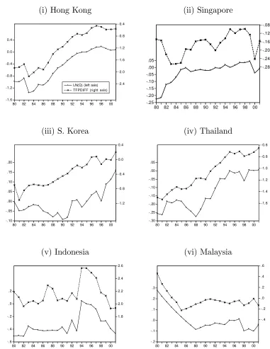
Figure 1 plots the relative price of nontradables and the (labor-share-adjusted)

12_{We test the homogeneity restriction using the Wald-test proposed by Mark, Ogaki and Sul}

(16)

sectoral TFP di¤erential within each country. For HK and Indonesia, the two series

move together very closely and virtually all of the medium to long-term changes in

the relative price of nontradables are matched by similar changes in the sectoral TFP

di¤erentials. However, for Singapore and Malaysia comovements between relative

prices and TFP di¤erentials appear to be smaller. Overall, the visual evidence of

Figure 1 appears to be consistent with the cointegration results documented above.

To summarize, the results of Table 4 provide reasonably strong con…rmation of

the …rst key prediction of the B-S model that the stochastic trend in sectoral TFP

di¤erentials can rationalize the stochastic trend in the relative price of nontradables.

The null hypothesis of no cointegration between the relative price of nontradables and

sectoral TFP di¤erentials can be rejected based on most cointegration tests when

the homogeneity assumption is maintained and by four out of six statistics when

heterogeneity is allowed for. Moreover, the unit value of the coe¢cient of the sectoral

TFP di¤erential also appears to be plausible under the homogeneity restriction.

4.4 PPP for Tradables

Table 5 reports the results of the tests for the assumption of long run PPP for tradable

goods. It is based on applying bootstrap cointegration tests to residuals obtained from

various regressions of the Asian countries’ tradable goods prices on U.S. tradable

goods prices adjusted for the nominal exchange rate.

The point estimates of the homogeneous cointegration vector are 1.31

(homoge-neous OLS) and 1.21 (PDOLS), and the unit value implied by the law of one price

cannot be rejected based on PDOLS standard errors. The estimated coe¢cients based

on heterogeneous OLS are positive for all countries except Singapore.

The upper section of Panel A reports the cointegration test results under the

(17)

no cointegration is rejected by …ve out of six test statistics at conventional signi…cance

levels. The lower section of Panel A reports the results of cointegration tests when

the homogeneous cointegrating vector assumption is relaxed. The null hypothesis of

no cointegration is again rejected by most of the six test statistics except for Kao’s

Dickey-Fuller t statistic. The OLS estimates for HK, Thailand and Malaysia are

1.26, 0.95 and 0.91 respectively, which are relatively close to the predicted unit value.

However, Singapore has a negative coe¢cient which contradicts the prediction of the

PPP relationship.

Overall, the statistical evidence for PPP for tradable goods is quite supportive

when the homogeneity restriction implied by the model is imposed but generally

weaker under heterogeneity. However, it should be noted that aggregating micro

data using CPI weights may increase the persistence of the median traded good. It is

thus possible that using disaggregated data can provide more favorable evidence for

PPP for tradable goods than is provided by our aggregated data.13

4.5 Real Exchange Rates

Table 6 reports the results for the second key prediction of the B-S model, which states

that the bilateral real exchange rates should be cointegrated with the composite TFP

di¤erential between the home country and the U.S. Analogous to Tables 4 and 5,

Panel A reports the cointegration test results while Panel B reports the estimates of

the cointegrating vectors. Under the homogeneous cointegration vector assumption

implied by the model, the estimated coe¢cients are 1.03 (homogeneous OLS) and

1.14 (PDOLS), which are remarkably close to the theoretically implied unit value.

13_{Crucini and Shintani (2008) document that the median traded good in the U.S. has a half-life}

(18)

Moreover, almost all cointegration tests reject the null hypothesis of no cointegration

at the 1 percent signi…cance level, except for Kao’s DF .

For the heterogeneous cointegration vector case, there is considerable disparity

across countries on the estimated coe¢cients of the composite productivity

di¤eren-tial. The coe¢cient of HK (1.0978) is close to the predicted unit value but less so

for other countries. Moreover, the results of the cointegration tests are rather mixed.

While Pedroni’s tests reject the null hypothesis of no cointegration, Kao’s tests do

not.14

To summarize the evidence for the second key prediction of the B-S model, there

is strong evidence of cointegration between real exchange rates and the composite

productivity di¤erential when the assumption of homogeneous cointegrating vector

is maintained. Moreover, the coe¢cient estimates are very close to the unit value

implied by the model. However, there is less accord for the heterogeneous case.

4.6 Real Exchange Rate Misalignment

As mentioned in the introduction, a natural by-product of the productivity-based

model is that it provides one with an estimate of the "long-run equilibrium real

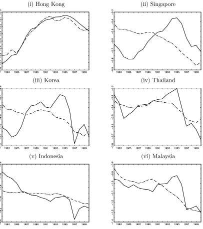
exchange rate" of the Asian real exchange rates against the U.S. dollar. Figure

2 plots the real exchange rates of the Asian countries against the U.S. dollar and

the estimated long run equilibrium values based on the PDOLS cointegrating vector

estimates reported in Panel B of Table 6. The …rst panel shows the results for Hong

Kong. The actual real exchange rate moves quite closely together with the implied

equilibrium value predicted by the model, although there is a modest undervaluation

in the early 1990’s and a modest overvaluation from 1993 onwards.

14_{The Wald test for the homogeneity restriction rejects the null hypothesis that the coe¢cients}

(19)

The second panel of Figure 2 shows the results for Singapore. The B-S model

predicts a sustained real depreciation of the Singapore dollar and it misses some of

the big swings in the actual real exchange rate. These results are consistent with the

earlier evidence suggesting that the basic ingredients of the B-S model – namely the

PPP for tradables and the close relationship between the real exchange rate and the

composite TFP di¤erentials – appear not to hold for Singapore.

The third panel shows the real exchange rate and the …tted value for Korea. The

model captures the major turning points of the actual real exchange rate, although

it underestimates the volatility of the real exchange rate. The real exchange rate

appears substantially overvalued in the years preceding the Asian …nancial crisis.

The fourth panel contains the results for Thailand. The model predicts a slight

depreciation of the real exchange rate over the entire sample. However, the actual

real exchange rate undergoes a continuous appreciation from the mid-1980’s up to

1995, followed by a massive depreciation.

The …fth panel shows the actual and …tted real exchange rates for Indonesia.

The model captures the secular depreciation of the real exchange rate over the entire

sample quite well. In sharp contrast to the other countries, the real exchange rate

appears to be undervalued in the years prior to the crisis.

The last panel shows the actual and …tted real exchange rates for Malaysia. The

real exchange rate ‡uctuates around its long-run equilibrium value, exhibiting an

undervaluation in the late 1980’s and an overvaluation in the 1990’s prior to the

crisis.

Table 7 shows the estimated average overvaluation during the three year period

prior to the crisis (1994 through 1996) and also at the end of 1996. At the eve of the

crisis in 1996 all countries except Indonesia show overvalued real exchange rates, with

Hong Kong being the least overvalued at 3.54% and Singapore the most overvalued

(20)

the extent of overvaluation ranging between 14% to 16%. Figure 2 also shows that

for all the countries except Indonesia, the real exchange rate overvaluation reached a

peak near 1995 and then the downward adjustment towards equilibrium commenced.

However, by 1996 panic had set in the region and the speculators were likely

ex-pecting large further declines. They therefore behaved in a way that resulted in the

declines they were expecting. Hence the real and nominal exchange rates depreciated

signi…cantly more than the required adjustment indicated by the productivity based

model. For instance, the real exchange rates of Korea, Thailand and Indonesia had

depreciated below its implied equilibrium value by 1997.

Viewed through the lens of the B-S model, it therefore seems plausible that both

fundamental factors and self-ful…lling expectations had a role to play in the Asian

…nancial crisis. The productivity based fundamental factors indicate large and

per-sistent overvaluations in the few years prior to the crisis.

5 Conclusions

This paper examined the evidence for a productivity-based explanation of the long

run real exchange rate movements for six Asian economies in the context of the

Balassa-Samuelson model. Relative to earlier studies, which are at best only weakly

supportive of the Balassa-Samuelson e¤ect, we …nd that sectoral TFP di¤erentials

play an important role in explaining the long term trends in both the relative price

of nontradables and the real exchange rates of these Asian countries.

These results are consistent with the view espoused in recent research that real

ex-change rates possess both permanent and temporary components. For instance, Mark

and Choi (1997) show that models in which the long-run real exchange rate is

identi-…ed as the permanent component of the real exchange rate outperform models which

(21)

that the real exchange rate contains an economically signi…cant component

associ-ated with the relative price of nontraded goods. In conjunction with recent work that

emphasizes the importance of nontradable goods in explaining long-run real exchange

rate movements (e.g. Burstein, Eichenbaum and Rebelo 2005a, Burstein, Eichenbaum

and Rebelo 2005b, Betts and Kehoe 2006, Crucini and Shintani 2008, Kakkar and

Ogaki 1999, and Park and Ogaki 2007), these results suggest that productivity

di¤er-entials may be an important factor in explaining the persistent departures of nominal

(22)

References

Alba, Joseph D., and David H., Papell. (2007) “Purchasing Power Parity and

Coun-try Characteristics: Evidence From Panel Data Tests,”Journal of Development

Economics, 83, 240-251.

Balassa, Bela. (1964) “The Purchasing-Power Parity Doctrine: A Reappraisal,”Journal

of Political Economy, 51, 584-596.

Bernanke, Ben., and Refet S., Gurkaynak. (2001) “Is Growth Exogenous?

Tak-ing Mankiw, Romer and Weil Seriously,”NBER Working Paper 8365, NBER,

Cambridge.

Betts, Caroline., and Timothy Kehoe. (2006) “U.S. Real Exchange Rate

Fluctu-ations and Relative Price FluctuFluctu-ations,”Journal of Monetary Economics, 53,

1297-1326.

Bosworth, Barry. (2005) “Economic Growth in Thailand: The Macroeconomic

Context,”The Brookings Institution.

Breitung, J½org. (2000) “The Local Power of Some Unit Root Tests for Panel

Data,”Advances in Econometrics, 15, 161-178.

Burstein, Ariel., Martin Eichenbaum, and Sergio Rebelo. (2005a) “Large

Deval-uations and the Real Exchange Rate,”Journal of Political Economy, 113(4),

742-784.

Burstein, Ariel., Martin Eichenbaum, and Sergio Rebelo. (2005b) “The

Impor-tance of Nontradable Goods’ Prices in Cyclical Real Exchange Rate

(23)

Chang, Yoosoon. (2004) “Bootstrap Unit Root Tests in Panels with Cross-Sectional

Dependency,”Journal of Econometrics, 120, 263-293.

Chang, Yoosoon., Joon Y. Park, and Kevin Song. (2006) “Bootstrapping

Cointe-grating Regressions,”Journal of Econometrics, 133, 703-739.

Cheung, Yin-Wong., and K. S., Lai. (2000) “On Cross-Country Di¤erences in the

Persistence of Real Exchange Rates,”Journal of International Economics, 50,

375-397.

Chinn, Menzie D. (1996) “Asian Paci…c Real Exchange Rates and Relative Prices,”

Manuscript, University of California, Santa Cruz.

Chinn, Menzie D. (2000) “The Usual Suspects? Productivity and Demand Shocks

and Asia-Paci…c Real Exchange Rates,”Review of International Economics,

8(1), 20-43.

Choudhri, Ehsan U., and Mohsin S., Khan. (2004) “Real Exchange Rates in

Devel-oping Countries: Are Balassa-Samuelson E¤ects Present?”IMF Working Paper.

Chow, Gregory C. (1993) “Capital Formation and Economic Growth in China,”The

Quarterly Journal of Economics, 108(3), 809-42.

Crucini, Mario J., and Mototsugu Shintani. (2008) “Persistence in Law of One

Price Deviations: Evidence from Micro-Data,”Journal of Monetary Economics,

55, 629-644.

De Gregorio, Jose., Alberto Giovannini, and Thomas Krueger. (1994) “The Behavior

of Nontradable Goods Prices in Europe: Evidence and Interpretation,”Review

(24)

De Gregorio, Jose., Alberto Giovannini, and Holger C., Wolf. (1994) “International

Evidence on Tradables and Nontradables In‡ation,”European Economic Review,

38, 1225-1244.

Drine, Imed., and Christophe Rault. (2002) “Does the Balassa-Samuelson

Hypoth-esis Hold for Asian Countries? An Empirical Analysis Using Panel Data

Coin-tegration Tests,”William Davidson Working Paper Number 504, The William

Davidson Institute.

Engel, Charles. (2000) “Long-run PPP May Not Hold After All,”Journal of

Inter-national Economics, 57, 243-273.

Feenstra, Robert., and Hiau Looi Kee. (2004) “On the Measurement of Product

Variety in Trade,”American Economic Review, 94(2), 145-149.

Garofalo, Gasper A., and Steven Yamarik. (2002) “Regional Convergence:

Evi-dence from a New State-by-State Capital Stock Series,”Review of Economics

and Statistics, 84(2), 316-323.

Gollin, Douglas. (2002) “Getting Income Shares Right,”Journal of Political

Econ-omy, 2002, 110(2), 458-474.

Im, Kyung So, M. Hashem Pesaran, and Yongcheol, Shin. (1995) “Testing for Unit

Roots in Heterogeneous Panels,” Manuscript, University of Cambridge.

_ _ _ _ _ _ _ (1997) “Testing for Unit Roots in Heterogeneous Panels,”

Manu-script, University of Cambridge.

_ _ _ _ _ _ _ (2003) “Testing for Unit Roots in Heterogeneous Panels,”Journal

(25)

Ito, Takatoshi., Peter Isard, and Steven Symansky. (1999) “Economic Growth and

Real Exchange Rate: An Overview of the Balassa-Samuelson Hypothesis in

Asia,”InChanges in Exchange Rates in Rapidly Developing Countries: Theory,

Practice and Policy Issues, edited by Takatoshi Ito and Anne Krueger, Chicago:

The University of Chicago Press.

Kakkar, Vikas. (2003) “The Relative Price of Nontraded-Goods and Sectoral Total

Factor Productivity: An Empirical Investigation,”Review of Economics and

Statistics, 85(2), 444-452.

Kakkar, Vikas., and Masao Ogaki. (1999) “Real Exchange Rates and Nontradables:

A Relative Price Approach,”Journal of Empirical Finance, 6, 193-215.

Kakkar, Vikas., and Isabel K. Yan. (2011) "Real Exchange Rates and Productivity:

Evidence From Asia", Working Paper, City University of Hong Kong.

Kao, Chihwa. (1999) “Spurious Regression and Residual-based Tests for

Cointegra-tion in Panel Data,”Journal of Econometrics, 90, 1-43.

Kim, J. I., and J. L., Lau. (1995) “The Role of Human Capital in the Economic

Growth of the East Asian Newly Industrialized Countries,”Asia-Paci…c

Eco-nomic Review, 1(3), 3-22.

Levin, Andrew., and Chien-Fu Lin. (1993) “Unit Root Tests in Panel Data: New

Results,”Working Paper, University of California, San Diego.

Li, Kui-Wai. (2002) “Hong Kong’s Productivity and Competitiveness in the Two

Decades of 1980-2000,” Working Paper, The City University of Hong Kong.

_ _ _ _ _ _ _ .(2006) The Hong Kong Economy: Recovering and Restructuring,

(26)

Maddala, G. S., and S. Wu. (1999) “A Comparative Study of Unit Root Tests

with Panel Data and a New Simple Test,”Oxford Bulletin of Economics and

Statistics, 61, 631-652.

Mark, Nelson C., and Donggyu Sul. (2003) “Cointegration Vector Estimation for

Panel DOLS and Long Run Money Demand,”Oxford Bulletin of Economics and

Statistics, 65, 655-680.

Mark, Nelson C., and Doo-Yull Choi. (1997) “Real Exchange-Rate Prediction Over

Long Horizons,”Journal of International Economics, 43, 29-60.

Mark, Nelson C., Masao Ogaki, and Donggyu Sul. (2005) “Dynamic Seemingly

Unrelated Cointegrating Regressions,”Review of Economic Studies, 72, 797-820.

Obstfeld, Maurice., and Kenneth Rogo¤. (1996)Foundations of International

Macro-economics, The MIT Press, Cambridge, Massachusetts.

Ortega, D., and F. Rodriguez. (2006) “Are Capital Shares Higher in Poor Countries?

Evidence from Industrial Surveys,”Wesleyan Economics WP, 23.

Park, Sungwook, and Masao Ogaki. (2007) “Long-Run Real Exchange Rate Changes

and the Properties of the Variance of k-Di¤erences,” Ohio State University

Working Paper #07-01, Department of Economics, Ohio State University.

Pedroni, Peter. (1999) “Critical Values for Cointegration Tests in Heterogeneous

Panels With Multiple Regressors,”Oxford Bulletin of Economics and Statistics,

November (Special Issue), 653-669.

Pedroni, Peter. (2004) “Panel Cointegration: Asymptotic and Finite Sample

Prop-erties of Pooled Time Series Tests with an Application to the PPP

(27)

Samuelson, Paul. (1964) “Theoretical Notes on Trade Problems,”Review of

Eco-nomics and Statistics, 46, 145-54.

Solow, Robert M. (1957) “Technical Change and the Aggregate Production

Func-tion,”Review of Economics and Statistics, 39, 312-20.

Stockman, Alan C., and Linda Tesar. (1995) “Tastes and Technology in a

Two-Country Model of the Business Cycle: Explaining International Co-movements”,

American Economic Review, 85(1), 168-85.

The Economist. (2009)Pocket World in Figures, Pro…le Books, London.

Thomas, Alastair, and Alan King. (2008) “The Balassa-Samuelson Hypothesis in

the Asia-Paci…c Region Revisited,”Review of International Economics, 16(1),

(28)

[image:28.612.92.543.123.430.2]

Table 1: Hong Kong: Unit Root Tests of Im, Pesaran and Shin (1995, 1997) and Breitung (2000)

Im, Pesaran and Shin (1995, 1997)d _Breitungd

IPS95 IPStrend95 IPS97 IPStrend97 IPSLM IPStrendLM (2000)

lnQb _0.8744 _0.3551 _0.8722 _0.3688 _-1.0057 _-1.5523 _-0.4530

bootstrap (0.8300)a _(0.5950) _(0.8300) _(0.5950) _(0.1650) _(0.1650) _(0.5550)

asymptotic (0.1909)a _(0.3612) _(0.1916) _(0.3561) _(0.1573) _(0.0603) _(0.3253)

d 0.8626 0.4829 0.8602 0.4995 -0.9979 -1.5458 -0.5264 bootstrap (0.7560) (0.6690) (0.7560) (0.6690) (0.2270) (0.2270) (0.5390) asymptotic (0.1942) (0.3145) (0.1948) (0.3087) (0.1592) (0.0611) (0.2993)

ln PU S

T E

c

-1.5263 -0.2133 -1.5727 -0.2124 1.7446 0.7661 1.2305 bootstrap (0.7340) (0.8140) (0.7340) (0.8140) (0.2660) (0.2660) (0.7790) asymptotic (0.0635) (0.4155) (0.0578) (0.4158) (0.0405) (0.2218) (0.1092)

ln (P_T) -1.5637 1.3803 -1.6108 1.4171 1.7914 0.8056 2.3871 bootstrap (0.4050) (0.7850) (0.4050) (0.7850) (0.5950) (0.5950) (1.0000) asymptotic (0.0589) (0.0837) (0.0536) (0.0782) (0.0366) (0.2102) (0.008)

ln (Er₎c

0.1353 0.9503 0.1194 0.9774 -0.3445 -0.9950 0.0866 bootstrap (0.6120) (0.8500) (0.6120) (0.8500) (0.3860) (0.3860) (1.0000) asymptotic (0.4462) (0.1710) (0.4526) (0.1642) (0.3652) (0.1599) (0.4655)

dC _0.3757 _0.8076 _0.3643 _0.8314 _-0.5949 _-1.2061 _-0.1620

bootstrap (0.6290) (0.7830) (0.6290) (0.7830) (0.3600) (0.3600) (0.5980) asymptotic (0.3536) (0.2097) (0.3578) (0.2029) (0.2759) (0.1139) (0.4356)

Notes: a _{P-values are in parentheses. *, ** and *** denote signi…cance at the 10%, 5% and 1%}

level respectively.

b _ln_Q_{stands for the log relative nontradable price.} _d_{refers to the labor-share-adjusted sectoral TFP}

di¤erential. ln PU S

T E refers to the log of the US tradable price times the nominal exchange rate.

ln (P_T)refers to the home tradable price. ln (Er₎_{denotes the log real exchange rate, and}_dC _denotes

the composite TFP di¤erential between the home and foreign countries.

c _{An Asian-crisis dummy is included to allow for a possible break in the nominal and real exchange}

Rate. The dummy equals 1 from 1997 onwards.

d _IPS

95refers to the average ADF test proposed by Im, Pesaran, and Shin (1995). IPS considers

the case that error terms are serially correlated.

IPS97 and IPS_LM are the ADF t and LM-bar tests suggested in Im, Pesaran, and Shin (1997),

respectively. The IPSLM statistics reported here are those that allow for serial correlation.

All IPS tests allow for heterogeneous unit root coe¢cients. The test statistics with superscript “trend” are performed on detrended data.

Breitung (2000)found the losses of power due to the bias correction terms in Levin and Lin

(29)

Table 2a: Hong Kong — Kao’s (1999) and Pedroni’s (1999) Cointegration Tests on the Regression of the Relative Price of Nontradables on the Sectoral TFP Di¤erentials

lnQ_HKt= + d_HKt+ t

Panel A: Cointegration Tests with OLS Estimation of the Cointegrating Vector Kao’s Testsa _{Pedroni’s Tests}b

DF DF_t ADF (1 lag) ADF (2 lags) P anel_t_p Gr_t_p

-3.0260 -2.1379 -3.3317 -3.5643 -2.6171 -2.7374 bootstrap (0.008)c _(0.000) _(0.000) _(0.000) _(0.000) _(0.000)

asymptotic (0.001) (0.016) (0.000) (0.000) (0.004) (0.003) Panel B: OLS Estimation of the Cointegrating Vector

bOLS

Coe¢cient 0.9016d

Table 2b: Hong Kong — Kao’s (1999) and Pedroni’s (1999) Cointegration Tests on the Regression of the PPP for Tradable Goods

lnP_{T ;HKt}= 0₊_'D

97_;t+ ln P_{T ;U St}E_HKt + 0_te

DF DF_t ADF (1 lag) ADF (2 lags) P anel_t

p Grtp

-3.2129 -1.9079 -0.9676 -0.9509 -0.1938 0.1392 bootstrap (0.602)c _(0.159) _(0.000) _(0.000) _(0.000) _(0.000)

bOLS

Coe¢cient 1.2625d

Table 2c: Hong Kong — Kao’s (1999) and Pedroni’s (1999) Cointegration Tests on the Regressions of the Real Exchange Rate on the Composite TFP Di¤erentials

lnEr

HKt= 00+'00D97;t+ dC_HKt+ 00t e

p Grtp

-3.2435 -2.4852 -2.5899 -3.6291 -1.8893 -1.8735 bootstrap (0.7880)c _(0.3480) _(0.000) _(0.000) _(0.000) _(0.000)

bOLS

Coe¢cient 1.0978d

a _DF _and_DF

t denote the bias-corrected Dickey-Fuller rho and t statistics of Kao (1999) respectively. b _{P anel}

tp andGrtp denote Pedroni’s (1999 and 2004) parametric panelt-statistic and parametric

groupt-statistic, respectively. The number of lags for each cross section is calculated according to the Akaike Information Criterion or Bayesian Information Criterion (AIC/BIC). The length of kernel window is calculated a la Andrews or Newey-West. For theP anel_t

p test, we use the estimate of the

long-run variance.

c _{P-values are in parentheses. *, ** and *** denote signi…cance at the 10%, 5% and 1% level respectively.} d _{Since the OLS standard errors are not valid for conducting inference, we do not report them here.} e_{An Asian-crisis dummy}_D

97is included to allow for a possible break in the nominal exchange rate.

(30)

[image:30.612.91.547.115.281.2]

Table 3: Panel Unit Root Tests of Im, Pesaran and Shin (1995, 1997) and Breitung (2000)

Im, Pesaran and Shin (1995, 1997)d _Breitungd

IPS95 IPStrend95 IPS97 IPStrend97 IPSLM IPStrendLM (2000)

lnQb _-0.6795 _1.1762 _-0.7369 _1.2166 _-2.8261 _-4.1084 _-0.4039

(0.9600)a _(0.9620) _(0.9600) _(0.9620) _(0.4390) _(0.4390) _(0.9940)

d -0.1953 -0.8073 -0.2438 -0.8115 -2.4916 -3.8264 -0.8943 (0.5400) (0.1570) (0.5400) (0.1570) (0.5940) (0.5940) (1.0000)

ln P_{T ;U S} E c -2.4585 0.4158 -2.5486 0.4392 -1.6133 -3.0856 -2.7027

(0.7120) (0.8050) (0.7120) (0.8050) (0.4560) (0.456) (0.9410)

ln (P_T) 0.6236 2.8670 0.5902 2.9455 -2.6584 -3.9671 3.7599 (0.6600) (0.9200) (0.6600) (0.9200) (0.2590) (0.2590) (1.0000)

ln (Er₎c _-0.8566 _1.5906 _-0.9173 _1.6404 _-2.9624 _-4.2234 _-0.5328

(0.6870) (0.9520) (0.6870) (0.9520) (0.2410) (0.2410) (0.030)

dC _2.8903 _1.2485 _2.8987 _1.2905 _-2.1066 _-3.5019 _-0.1939

(0.8110) (0.7990) (0.8110) (0.7990) (0.3430) (0.3430) (1.0000) Notes: a _{Bootstrap p-values are in parentheses. *, ** and *** denote signi…cance at the 10%, 5% and 1%}

level respectively.

b _ln_Q_{stands for the log relative nontradable price.} _d_{refers to the labor-share-adjusted sectoral TFP}

di¤erential. ln P_{T ;U S} E refers to the log of the US tradable price times the nominal exchange rate.

ln (P_T)refers to the home tradable price. ln (Er₎_{denotes the log real exchange rate, and}_dC _denotes

the composite TFP di¤erential between the home and foreign countries.

c _{An Asian-crisis dummy is included to allow for a possible break in the nominal and real exchange rate.}

The dummy equals 1 from 1997 onwards.

d _IPS95_{refers to the average ADF test proposed by Im, Pesaran, and Shin (1995). IPS allows}

for a heterogeneous coe¢cient ofyi;t 1 and considers the case that error terms are serially

correlated with di¤erent serial correlation coe¢cients across cross-sectional units.

IPS97 and IPSLM are the ADF t and LM-bar tests suggested in Im, Pesaran, and Shin (1997),

respectively. The IPSLM statistics reported here are those that allow for serial correlation.

All IPS tests allow for heterogeneous unit root coe¢cients. The test statistics with superscript “trend” are performed on detrended data.

Breitung (2000)found the losses of power due to the bias correction terms in Levin and Lin

(31)

[image:31.612.95.544.341.503.2]

Table 4: Kao’s (1999) and Pedroni’s (1999) Cointegration Tests on the Regression of the Relative Price of Nontradables on the Sectoral TFP Di¤erentials

Panel A: Cointegration Tests

Based on OLS Estimation with Homogeneous Cointegrating Vectore

lnQit= i+ dit+it

Kao’s Testsa _{Pedroni’s Tests}b

DF DF_t ADF(1 lag) ADF(2 lags) P anel_t

p Grtp

statistic -4.3765 -6.2549 -6.0048 -3.2566 0.3553 -1.3632 p-value (0.000) c _(0.106) _(0.000) _(0.000) _(0.003) _(0.000)

Based on OLS Estimation with Heterogeneous Cointegrating Vectore

lnQit= i+ idit+ it

Kao’s Tests Pedroni’s Tests

p Grtp

statistic -18.4535 -9.2445 -5.9251 -1.9814 -2.3103 -2.9531 p-value (0.006) (0.000) (0.451) (0.999) (0.000) (0.000)

Panel B: Estimation of the Cointegrating Vector

OLS with Homogeneous Cointegrating Vectore

lnQit= i+ dit+it

bOLS 0.6399d

OLS with Heterogeneous Cointegrating Vectore

lnQit= i+ idit+ it

HKf _SIN _KOR _{T HA} _{IN D} _{M AL}

bOLS_i 0.9016d _0.4368 _0.1303 _0.3159 _0.7569 _0.5457

Mark and Sul (2003)’s PDOLS

lnQit= i+ dit+it

bP DOLS 0.688

S.E. (parametric s.e.: 0.235, Andrews s.e.: 0.196)

a _DF _and_DF

groupt-statistic, respectively.

c _{Bootstrap p-values are in parentheses. *, ** and *** denote signi…cance at the 10%, 5% and 1% level}

respectively.

d _{Since the OLS standard errors are not valid for conducting inference, we do not report them here.} e_{The cointegrating vectors are estimated using OLS with country-speci…c …xed e¤ects.}

f _{“HK”, “SIN”, “KOR”, “THA”, “IND” and “MAL” refer to Hong Kong, Singapore, S. Korea, Thailand,}

(32)

Table 5: Kao’s (1999) and Pedroni’s (1999) Cointegration Tests on the Regression of the PPP for Tradable Goods

lnP_{T ;it}= 0

i+'D97_;it+ ln P_{T ;U St}E_it + 0_it g

statistic -11.556 -8.9464 -5.3346 -5.0509 0.1302 0.7766 p-value (1.000)c _(0.017) _(0.000) _(0.000) _(0.009) _(0.000)

lnP_{T ;it}= 0

i+'iD97_;it+ _iln P_{T ;U St}E_it + 0_it

p Grtp

lnP_{T ;it}= 0

i+'D97_;it+ ln P_{T ;U St}E_it + 0_it

bOLS 1.3121d

lnP_{T ;it}= 0

i+'iD97_;it+ _iln P_{T ;U St}E_it + 0_it

bOLS_i 1.2625d _-0.1427 _0.6589 _0.9530 _1.9459 _0.9102

lnP_{T ;it}= 0

i+'D97_;it+ ln P_{T ;U St}E_it + 0_it

bP DOLS 1.213

a _DF _and_DF

respectively.

Indonesia and Malaysia respectively.

g _{An Asian-crisis dummy}_D

97 is included to allow for a possible break in the nominal exchange rate.

(33)

[image:33.612.94.545.342.511.2]

Table 6: Kao’s (1999) and Pedroni’s (1999) Cointegration Tests on the Regression of the Real Exchange Rate on the Composite TFP Di¤erentials

lnEr

it= 00i+'00D97_;it+ dC it+

00 it g

lnEr

it= 00i+'00iD97_;it+ id

C it+ 00it

p Grtp

lnEr

it= 00i+'00D97_;it+ dC it+

00 it

bOLS 1.0296d

lnEr

it= 00i+'00iD97_;it+ id

C it+ 00it

bOLSi 1.0978d -0.6896 -0.9880 2.0016 4.7100 0.2750

lnEr

it= 00i+'00D97;it+ dC_it+00it

bP DOLS 1.144

a _DF _and_DF

respectively.

Indonesia and Malaysia respectively.

g _{An Asian-crisis dummy}_D

97 is included to allow for a possible break in the nominal exchange rate.

(34)

[image:34.612.131.481.120.206.2]

Table 7

Estimated Real Exchange Rate Misalignment

Country Average Overvaluation during 1994-96 Overvaluation in 1996 Hong Kong 3.79% 3.54%

(35)

(i) Hong Kong (ii) Singapore -1.6 -1.2 -0.8 -0.4 0.0 0.4 -2.4 -2.0 -1.6 -1.2 -0.8 -0.4

80 82 84 86 88 90 92 94 96 98 00 LN(Q) (left axis) TFPDIFF (right axis)

-.25 -.20 -.15 -.10 -.05 .00 .05 -.28 -.24 -.20 -.16 -.12 -.08

80 82 84 86 88 90 92 94 96 98 00

(iii) S. Korea (iv) Thailand

-.10 -.05 .00 .05 .10 .15 .20 -1.2 -0.8 -0.4 0.0 0.4

80 82 84 86 88 90 92 94 96 98 00

-.30 -.25 -.20 -.15 -.10 -.05 .00 .05 -1.6 -1.4 -1.2 -1.0 -0.8 -0.6

80 82 84 86 88 90 92 94 96 98 00

(v) Indonesia (vi) Malaysia

-.6 -.4 -.2 .0 .2 1.8 2.0 2.2 2.4 2.6

80 82 84 86 88 90 92 94 96 98 00

-.2 -.1 .0 .1 .2 .3 -.4 -.2 .0 .2 .4 .6

[image:35.612.111.492.82.575.2]

80 82 84 86 88 90 92 94 96 98 00

(36)

(i) Hong Kong (ii) Singapore

(iii) Korea (iv) Thailand

[image:36.612.101.507.88.547.2]

(v) Indonesia (vi) Malaysia