Munich Personal RePEc Archive
Asset price, asset securitization and
financial stability
Liu, Luke
China Economics and Management Academy, Central University of
Finance and Economics, Beijing, China
9 July 2011
Online at
https://mpra.ub.uni-muenchen.de/35000/
1
Asset Price, Asset Securitization and Financial Stability
Luke Liu1
Abstract: Prior to the Global Financial Crisis in 2008, securitization has been widely perceived as a way to disperse credit risks, and to enhance financial system’s capacity in dealing with defaults. This paper develops a model of securitization and financial stability in
the form of amplification effects. This model has illustrated three different scenarios: A
negative shock in the economy will lead to downturn of the economy and falling of the asset
prices, deteriorating balance sheets and tightening financing conditions. However, if there is
no shock or a positive shock, banks can improve its profitability significantly through
securitization. While securitization decreases the probability of systemic crisis, banks tend to
suffer more when the crisis happens as a result of over-borrowing and over-investing. This
paper uses a three-period theoretical model to demonstrate the impact of securitization on the
financial stability, and provides clear analytical guidelines for a new regulatory framework of
securitization that account for systemic risk and systemic externalities.
Key words: Asset Price; Asset Securitization; Systemic Risk; Financial Stability
2
Asset Price, Asset Securitization and Financial Stability
1 Introduction
The financial crisis started in the US in 2007 quickly spread out to all developed and
emerging economy, and is considered as the most serious crises since the Great Depression. Its global effects include the failure and bailout of key financial institutions, the decline in private wealth, substantial financial commitments incurred by many governments, and a significant decline in economic activities. This crisis raised the need for the researchers and policymakers around the globe to take unprecedented policy measures to deal with systemic risks (Gorton 2008, Brunnermeier 2009, Diamond and Rajan 2009, Blanchard 2009 and Krishnamurthy 2009). There is no coherent definition for systemic risk, but most existing research considers it as the danger or probability that financial institutions become insolvent in a large scale. This concept is different from so-called ―systematic risk’ which sometimes called market risk, aggregate risk, or undiversifiable risk, is the risk associated with aggregate market returns.
Comparing to the crisis in the 20th century, the recent crisis has three main features. Firstly, the immediate cause or trigger of the crisis is neither the bankruptcy of traditional banks nor currency crisis in the traditional sense, but the burst of the United States housing bubble which peaked in approximately 2005–2006. Secondly, the asset lead to crisis is not the long term investment project as before, but the mortgage-backed security (MBS). Thirdly, in order to keep liquidity, the financial institutions made panic selling of securities, which sharpened the severity of the crisis.
The fore-mentioned features of the crisis are associated with the operating model of the modern banking. Traditionally, the main source of bank’s revenue is interest on the capital it lends out to customers. And the bank profits from the difference between lending and deposit interest, as shown in figure 1.
Under the traditional banking model, the arrival of some negative information on banks' investment returns may lead to severe bank runs. There is a large range of research related to this issue. For example, Corrado(2005) analyse how a supranational institution which acts as an international lender of last resort can cope with banking crises by guaranteeing run-proof bank deposit contracts in the traditional banking crisis.
In the past decades, banks, especially American banks, have adopted different measures to remain profitable in a rapidly changing financial system. One popular measure adopted by large modern banks is to participate in financial markets by originating and distributing securities as well as operating in the monetary market. Originally, the securitization market served as a source of financing and many assumed that securitization would provide a more resilient source of financing compared with the conventional market that depends on
Depositor
s
Bank Borrower
$ $
[image:3.595.79.465.498.539.2]Insured Savings Mortgages
3
borrowing from other financial intermediaries. Figure 2 shows the structure of the securitized banking system.
Through securitization, banks can increase their leverages. Securitization can offer perfect matched funding by eliminating funding exposure in terms of both duration and pricing basis. Apart from these advantages, the securitization can also help banks to reduce capital
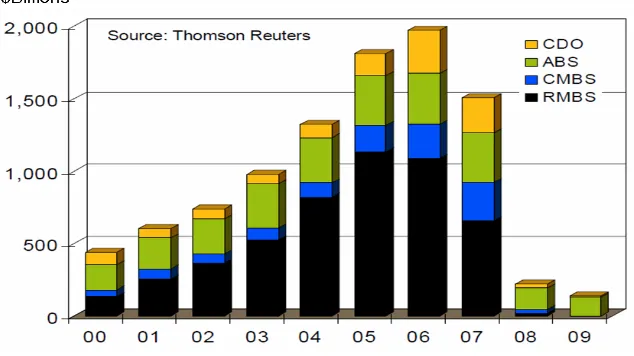
[image:4.595.69.538.114.234.2]requirements, lock in profits, and transfer risks. Given those benefits, it is not surprising that securitization has grown rapidly in banking industry. As shown in Figure 3, private bond issuance of residential and commercial mortgage-backed securities (RMBS and CMBS), asset-backed securities (ABS), and collateralized debt obligations (CDOs) peaked in 2006 to nearly $2 trillion. In 2009, private issuance dropped to less than $150 billion, and almost all of it was asset-backed issuance supported by the Federal Reserve's TALF (Term Asset-Backed Securities Loan Facility) program to aid credit card and small-business lenders.
Figure 3: Securitization market in U.S ($ billions)
Does securitization lead to the financial stability? It is difficult to answer this question without formally modelling the underlying externalities associated with systemic financial crises. This paper attempts to model the impact of asset securitization on financial systemic risk. We measure the likelihood of a crisis by the probability that a bank liquids all its asset, and its scale (impact) in terms of the asset price. Lower asset prices correspond to more serious crises.
Leverage is another important factor to consider on the financial stability and securitization is
Investors $ Bank Borrower
$
Mortgages Direct
Lenders Securitization
$ $
Mortgages Collateral
M
o
rt
g
ag
e
[image:4.595.133.450.430.608.2]s
4
crucial in understanding the leverage of the financial system as a whole. Securitization enables credit expansion through higher leverage of the financial system as a whole. If the expansion of assets entailed by the growth in financial system leverage drives down lending standards, securitization may decrease financial stability rather than promoting it.
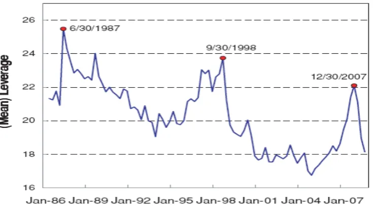
Figure 4 plots the leverage US primary dealers: First, leverage tends to decrease overall since 1986. This decline in leverage is due to the bank holding companies in the sample—a sample consisting only of investment banks shows no such trend in leverage (see Adrian and Shin, 2007). Secondly, each of the peaks in leverage was immediately followed by a financial crisis (the peaks are 1987Q2, 1998Q3, 2008Q3). Financial crisis tend to follow marked increases of leverage.
Source: SEC 10-K and 10-Q filings, sited in ―Leverage, Securitization and Global Imbalances‖
[image:5.595.117.485.219.422.2]Note: the set of 18 banks that has a daily trading relationship with the Fed. They consist of US investment banks and US bank holding companies with large broker subsidiaries (such as Citigroup and JP Morgan Chase)
Figure 4: Mean Leverage of US Primary Dealers
More research is needed on the links between bank leverage and the securitization. In our model, banks make, securitize, distribute, and trade asset good, or they hold consume good. They also borrow capital good, using their security holdings as collateral, which will form different leverages. And we then examine the relationship between security, leverage and financial stability.
Our model predicts that asset securitization makes crises less likely since banks have more consume good to keep liquid by asset securitization. As a result, direct lenders are more willing to lend, allowing banks to increase their borrowing and initial investment. But, if a crisis does occur, losses will be greater. Overall, asset securitization may serve as a measure to reduce the likelihood of crises but to magnify their potential impact.
The paper proceeds as follows. Section 2 reviews the related literature. Section 3 sets up the benchmark model. Section 4 shows the model with securitization. Section 5 concludes the paper. The Appendix contains all the proofs.
2 Related Literature
5
attempt to combine these three strands by describing banks’ choices of securitization and financial leverage as well as the impact on financial stability.
2.1 Asset prices and financial stability
The idea that the asset price influences on financial constraint and financial stability can be traced back at least as far as Veblen (1904, chap. 5), who described the positive interactions between asset prices and collateralized borrowing. Later, many researchers followed his idea and built up a large body of literature in this area. Bernanke and Gertler (1989), for example, construct an overlapping generation model in which financial market imperfections cause temporary shocks in net worth, and such shocks are to be amplified and to persist. In their model, a positive technology shock increases the labour demanded by the entrepreneurs who have been funded, and allows for more projects to be undertaken. Moreover, the
accompanying rise in wage improves the financial position of the next generation of
entrepreneurs, so more of their projects will be funded. They will subsequently demand more labour, and the cycle goes on. Kiyotaki and Moore (1997) extend the Bernanke and Gertler’s story by illustrating the positive feedback through asset prices and the associated
intertemporal multiplier process. During a business cycle, a major channel for shocks to net worth is through changes in the values of firms’ assets or liabilities. Asset prices reflect future market conditions. When the effects of a shock persist (as in Bernanke and Gertler 1989), the cumulative impact on asset prices, and hence on net worth at the time of the shock, can be significant. They show that small, temporary shocks to technology or income distribution can generate large, persistent fluctuations in output and asset prices.
Similar to Kiyotaki and Moore (1997), Lorenzoni (2008) studies the welfare properties of competitive equilibria in an economy with financial frictions hit by aggregate shocks. In particular, it shows that competitive financial contracts can result in excessive borrowing ex ante and excessive volatility ex post. The model provides a framework to evaluate preventive policies, which can be used during a credit boom to reduce the expected costs of a financial crisis. Existing studies allow for state-contingent financial contracts. However it is unclear to what extent the underlying externality drives their results. In contrast, our model compares the difference of the over borrowing rate with or without securitization between the actual financial contract and the state-contingent financial contracts which is clearer. Qiu(2011) build a general equilibrium model to analyze how the ability of banks to create money can affect asset prices and financial stability. His research focuses on the monetary policy while our research puts more attention to the relationship between asset price and asset
securitization.
2.2 Asset securitization and financial stability
Traditional theories of financial intermediation describe banks as accepting deposits,
6
of default, securitization weakened lenders’ incentives to screen borrowers, exacerbating the potential information asymmetries which lead to problems of moral hazard.
Using Bank Lending Survey, Maddaloni and Peydró (2009) study the determinants of bank lending standards in the Euro Zone, and find that high securitization activity amplifies the positive impact of low short-term interest rates on bank risk-taking. Using a large data set of securitized subprime loans in the U.S., Keys et al.(2009) find that loans originated by banks tend to default more relative to independent lenders. Their conclusions are well supported by Purnanandam(2008) and Loutskina and Strahan ( 2008). A central question surrounding the current subprime crisis is whether the securitization process reduced the incentives of financial intermediaries to carefully screen borrowers. Keys et al. (2010) examine this issue using data on securitized subprime mortgage loan contracts in the United States. Their findings suggest that existing securitization practices did adversely affect the screening incentives of subprime lenders. Although lots of empirical research shows the relationship between securitization and financial stability, there is little theoretical research in this area. We compare the securitization model to the benchmark model and test the validity findings of the empirical research.
2.3 Financial leverage and financial stability
Finally, this study is related to the extensive literature on leverage and financial systemic risk. Geanakoplos (1997, 2003) introduced the idea of endogenous margins or equilibrium
leverage. Geanakoplos (2003) especially identified increasing volatility and increasing disagreement as causes of increased margins, and hence of the leverage cycle. Adrian and Shin (2008) put forward a theory of pro-cyclical leverage and credit availability based on the optimizing behaviour of financial intermediaries. In their model, pro-cyclical leverage comes from investment bank’s focus on value at risk. Adrian and Shin argued that volatility is countercyclical, allowing banks to take more leveraged bets when asset prices are high.
Our approach is to build on Kiyotaki and Moore (1997) with three key differences.
First, we focus on asset securitization and its effect on financial leverage and systemic risk. In contrast, Kiyotaki and Moore (1997) focus on the dynamic interaction between credit limits and asset prices. Focusing on securitization allows us to closely explore its impact on financial leverage and systemic risk. Second, Kiyotaki and Moore (1997) analyse the
economic shock on net value and asset price through linearization. In this study, we calculate the equilibrium and then analyse the impact on the two factors. This allows us to illustrate the results in a more intuitive way. Third, Kiyotaki and Moore (1997) construct an economy with indefinite periods while we consider a model with just three periods, so as to make the model simpler as well as illustrating the impact of shock.
Another closely related paper is Shleifer and Vishny (2010). They also look at banks’
endogenous choice of liquidity which involves fire sales of illiquid assets. However, there are two major differences between our model and theirs. First, while their research only
7
3 The Benchmark Model
We consider a model with three periods: 0(initial period), 1(intermediate period), and 2(final period). The economy produces two goods, consumption good and capital good.
Consumption goods can be turned into capital goods on one for one basis at any point of time by the bankers, but the opposite is not feasible. There are two important assumptions. Firstly, we assume there are two types of players in the economy: bankers and direct lenders. They are risk neutral and identical within their group. Secondly, we assume the complete
competition in the banking industry following similar practice in Allen and Gale (1998), Rochet andVives (2004), and Korinek (2008). Free entry into the banking industry forces banks to compete by offering deposit contracts that maximize the expected utility of the firms. Thus, the bankers in our model can also be interpreted as entrepreneurs -in a sense that they make financing decisions and are subject to business risk.
Both the banker and direct lender can produce consume good and are indifferent to consume in period 0, 1, 2. At period 0, 1, 2, the respective expected utilities of a banker and a direct lender are 0b1b2b
and 0c1c2c
. There is no discounting and here is no interest
conflict between the bank owners and the bankers. The objective functions of a banker and a direct lender are:
Max 0( 0b 1b 2b)
E and Max 0( 0c 1c 2c)
E (1)
3.2 Endowments and Projects
Each banker has an endowment n of consumption goods at the beginning of his life and receives no further endowment in the following periods. Each direct lender receives a constant endowment e of consumption goods in each period.
Each direct lender owns a firm in the ―traditional sector‖. Firms in the traditional sector invest capital k1Ts in period 1 to produce consumption goods in period 2. The technology of the traditional sector is represented by the production function ( 1T)
s
G k . The function is increasing, strictly concave, twice differentiable and satisfies the following properties:
(0) 0
G , G'(0) 1 .
At the period t=1, there is a competitive spot market in which the consume good is exchanged for capital good at a price of q1s.The other market is a one-period credit market in which one
unit of consume good at period t=1 and t=2, is exchanged for a claim to R(R is a positive constant with the value no less than 1) units of consume good at period t=1 and t=2. For simplicity, we assume that the economy begins with no capital, so the price of capital is one at period 0, as long as some investment takes place.
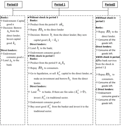
Figure 5 depicts the timeline of events. The banker has access to the following technology. In period 0, they choose the level of investment k0. In period 1, this investment yields a k1s 0
8
capital stock for next period, k1s , by making the net investment
1s 0
k k (k1s k0 0 means the banker sell part of his capital good). The capital stock k1s produces Ak1s units of
consumption goods in period 2, with A >R> 1. Capital fully depreciates at the end of period 2. To maximize his consumption, the banker can lend from the direct lenders bt and repay Rbt
in the period t+1(t=0,1). Both the banker and the direct lender can consume all the capital or consume good left in period 2. Since the economy ends at period 2, so there is no debt after period 2.
Let E(a1s) >R, so that early investment in period 0 is expected to be profitable. If a1s turns
out to be less than 1, the bank has two options: it can either sell a portion of its capital to direct lenders and continue with the investment project; or it can go into liquidation, abandoning the project and selling all of its capital to direct lenders.
Banks:
Endowment: Capital good n
Decision: Borrow
0
b from the direct lender; Invest capital good k0
Direct lenders:
Endowment consume good e
Lend b0 to the bank
●Without shock in period 1 Banks:
Product from the period 0: ak0
Repay Rb0 to the direct lender
Decision: Borrow b1 from the direct lender; Buy new capital good (k1k0)
Direct lenders:
Lend b1 to the bank;
Endowment consume good e ●With shock in period 1
Banks:
Product from the period 0 a k1s 0
Repay Rb0 to consumers.
Go to liquidation, or sell k1Ts capital to the direct lender, or make an investment and borrowb1s from the direct lender.
Direct lenders:
Lend b1s to banks. If there are fire sales (
1 0
T s k ),
invest (k1Ts) in traditional sector.
Endowment consume good e
Buy asset good k1Ts from the banker and invest it to the traditional sector.
●Without shock in period 1
Banks:
Repay Rb1 to the direct lender.
Consume all the goods left.
Direct lenders:
Consume all the goods left. ●With shock in period 1(The bank survives from the shock in period 1.)
RepayRb1s to consumers.
Consume all the goods left.
C Direct lenders:
Endowment consume good e
Consume all the goods left.
[image:9.595.77.495.291.727.2]Period 0 Period 1 Period2
9 3.4 Equilibrium with no shock
We now solve for equilibrium with no shock. Since direct lenders expect investment in the productive sector of the economy to be profitable and, since they have very large
endowments relative to bankers, they always meet the borrowing demands of the banker.
If the banker has capital good kt at the beginning of the period, then he can borrow t
b in total, as long as the repayment does not exceed the market value of his capital goods at period t+1(t=0,1), i.e.
0 0
0b
q n and 0 b1
q k1 0 (2)The two constraints specify that the banker can only borrow up to a fraction
of the value of their assets in each period, where we define
to be the maximum loan-to-value ratio as in Jermann and Quadrini (2006) and Gai et al. (2006). Since the economy ends at period 2, the banker has no incentive to borrow at period 2.The banker can expand his scale of production by investing in more capital goods. We consider a banker who holds endowment capital good n and has incurred a total debt b0. At the beginning of the period, he can invest k0 which should satisfies
0 0
k n b (3)
At period 1 the banker harvests ak0 capital good, which, together with a new loan b0, is available to cover the cost of buying new capital good, and to repay the accumulated debt
0
Rb (which includes interest). The banker’s flow-of-funds constraint at the period 1 is thus
1( 1 0) 0 0 1
q k k Rb ak b (4)
For the direct lender, without buying asset good from the fire sale of the banker, the direct lender would choose the debt '
0
b and ' 1
b lends to the banker to maximize the utility.
' ' ' '
0 0 1 1
( )
Max e b e Rb b e Rb i.e. ' '
0 1
[3 ( 1) ( 1) ]
Max e R b R b (5)
Market equilibrium is defined as a sequence of capital good prices and allocations of capital good, debt, and consumption, such that the banker maximizes the expected discounted utility (1) subject to the borrowing constraint (2) and the flow-of-funds constraint in period 0 and period 1; Each direct lender maximizes the expected discounted utility (1); and the markets for capital good and debt clear.
10
Lemma 1.
In equilibrium, asset prices are characterized by the conditionsqs G k'( sT), 1 ( 0 1 )
T
s s
k k k
for any state s.
From this lemma, it follows that two cases are possible in the capital market. In the first case, the price of capital is one, the traditional sector chooses no investment, and the
entrepreneurial sector makes positive investmentk1s k0 0. While in the second case, the price of capital '( T)
s s
q G k and the traditional sector chooses investmentk0k1s 0.
With these conditions, we can obtain proposition 1 which gives a characterization of optimal financial contracts between the banker and direct lender without economic shock.
Proposition 1.
In equilibrium without economic shock:
0 1 1
q q
,
0
b
nk0 (
1)n b1
( 1)n k1 (
1)(a
1)n
nR0 1 0
b b
2 1 1 [( 1)( 1) ] ( 1)
b
Ak b R A a n nR nR
The total consume of the direct lender would be 3 ( 1) ( 1) ( 1)
c
T e R n R n
Proof can be found in the Appendix. The intuition behind Proposition 1 is simple. Without shock in period 1, the output of period 0 is ak0 with certain. So the banker will borrow as much as possible. The banker and the direct lender reach the goal to maximize their utility. And we can see that, caeteris paribus, the consumption of the banker increases with a and
( 2 0b
a
and 2 0
b
), and the consume of the direct lender increases with
.3.5 Equilibrium with shock
In this section, we solve for the competitive equilibrium by considering the optimization problem of the representative banker. Under the economic shock, the representative banker’s optimization problem is given by:
0 0,1,2
max b
t t
E
Subject to:
0 0
k
n b
(6)1s
(
1s 0)
0 1s 0 1s11
1 1 1 0
b
s q ks s Rb
Vs: total liquidation in period 1 (8)
2 1 1
b
s Aks Rbs
Vs: partial or no liquidation (9)
2 0
b s
Vs: total liquidation in period 1 (10)
0 0
0b
q n(11)
1 1 0
0bsq ks (12)
Equation (6) represents the banker’s budget constraint in period 0: investment costs and any profits taken by the banker in period 0 must be financed by its endowment (initial net worth) and borrowing from direct lenders. In period 1, provided that the investment project
continues (i.e. provided that the bank does not go into total liquidation), the bank’s budget constraint is given by (7): Financing is provided by the start of the period assets at their market value and net period 1 borrowing, adjusted for the revenue surplus or shortfall. In period 2, profits are then given by (9).
By contrast, if the bank goes into total liquidation in period 1, it sells all of its capital at the market price, yielding q k1s 1 in revenue. Therefore, its period 1 profits are given by (8), while
period 2 profits are zero. Finally, (11) and (12) simply represent combined and simplified versions of the borrowing constraints.
Since the expected returns on investment are always high, it is clear that the bank will never take any profit until period 2 unless it goes into total liquidation. Therefore,
0
1s 0 for all state s. Moreover, given that the high return between periods 1 and 2 is certain, banks wish to borrow as much as possible at period 1. So (12) binds at its upper bound and b0
q n0 . Finally, the asset price is only endogenous in period 1: q0 1 because of the large supply of consumption goods in period 0 and no capital good sale.Proposition 2 shows the optimal financial contracts between the banker and the direct lender with economic shock in period 1.
Proposition 2. There exists a unique symmetric competitive equilibrium. In equilibrium, asset
prices satisfy0q1s 1. Depending on the shock a1s , the optimal debt is one of the following types:
Type1: a1sq1s R
0 1s 1s( 1s 1s) 1s 1s( 1s 1s ) 0
Z Z RZ a q Z RZ a q R
Then optimum b =0, in this case the bank will go to bankrupt or keep insolvent by 0* liquidating part of capital good. The over borrowing rate is
.Type2: a1sq1s R
0 1s 0
12 Then optimum *
0 (0, 0 )
b q n , in this case the bank will liquidate part of his capital good to keep insolvent. The over borrowing rate lies within the pale of (0,
).Type3: a1sq1s R
0 1s 0
Z Z R
Then optimum debt *
0 0
b q n, which is similar with the equilibrium without shock
Where 0 1 1
1
( s s)
s A
Z a q
q
and 1
1
s s A Z
q
. The over borrowing rate is 0.
The variables Z0and Z1s defined above, respectively, are the Lagrange multipliers on the
budget constraints at periods 0 and 1; they represent the rates of return on bank wealth in periods 0 and 1.The banker must exhaust his borrowing capacity in the high state
(a1sq1s R) while must borrow nothing in the low state(a1sq1s R). In the media state (a1sq1s R), the banker is indifferent between borrow any from the direct lender.
Obviously, in the low and media state, the banker is over borrowing ( *
0 0 0
b q nb ). As 1
( s)
E a R, the banker in the market aiming at maximum profit will always exhaust his borrowing capacity. The over borrowing rate in the low state is higher than in the media and high state.
Then we focus on the critical point that the bank liquidates all the capital good and the asset price. Using the result that the financial constraint is always binding in period 2 (from Appendix C), we can get
1 0 1 0 1 0 1
(ksk q) sb Ra ks bs
(13) Let 0 1 1T
s s
k k k , we can get
0 1 0 1
1
1
s s
s T
s b R a k b q
k
(14)
For b1s
q k1s 0, we can rewrite it as1 1
1
( 1) (1 )
s
s T
s
nR a n
q
k n
(15)
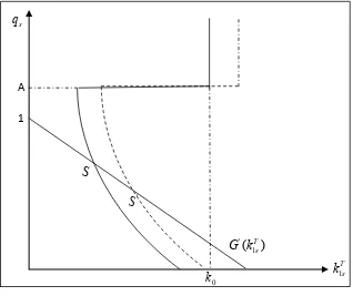
Equation (15) shows that the more assets the banker sells, the more deeply decreasing the asset price will be. Figure 6 gives a graphical illustration of the equilibrium in the state of low and media states for given values of k0, b0and b1s. Curve S plots the banker’s supply of
13
An increase in b1s increases the capital stock at period 0. The choice of b0affects the equilibrium price in another way. Figure 6 shows the effect of an increase in borrowing in period 0, leading to a rightward shift of the banker’s supply and to a lower equilibrium price.
For completeness, the figure includes the regions where q1s A arise in equilibrium although
such prices never arise in equilibrium as when q1s goes above A, the banker’s investment
becomes unprofitable and will sell all the capital good k0.
If the banker can’t make the repayment in period 1, then the bank will go bankrupt. There exist two extreme cases:
Case 1: No capital good sale. In this case, there is a positive shock that allows the banker to make the repayment in period 1 without fire sale.
1s 0 0
k k
From lemma 1, we can clearly find that
' 1
(0) s 1
G q . Letk1s k0 and we can get the
threshold for a1sfrom (13), which can be rewritten as
0 1s 0 1s
b Ra k b
(16)
Let b0
n and b1s
q k1s 0 into (16). We can get * 11
s
a R
. So we can see for any *
1s 1s a a
, there will be no fire sale. 1
s
[image:14.595.141.459.203.470.2]q
Figure 6 Asset market equilibrium 0
k 1
T s k '
S
S
A
' 1 ( T)
14
Case 2: Financial crisis. In this case, there is a negative shock that leads the representative
banker to sell all the capital good and still can’t keep solvent. Letk1s 0 and we can get the threshold for a1sfrom (13).
0 1s 0 1s 0 1s
b Ra k b k q (17)
Let b0
n and b1s
q k1s 0 into (17). We can get **1 1 1
1
s s s
a R q q
. For q1s G k'( )0 , we can get
** ' '
1 ( )0 ( )0
1
s
a R G k G k
. So we can see for any
' '
1 ( )0 ( )0
1
s
a R G k G k
, the bank will surely go bankrupt.
From figure 7, we can see clearly that the shock can directly have effect on asset price. When *
1s 1s
a a , there will be no asset sale and 1s 1
q . When **
1s 1s
a a , the bank will sell all the
capital good and ' 1s ( )0
q G k . With securitization, the threshold will be smaller. But when a
crisis happens, the loss will be larger than the situation without securitization which we will show in next section.
4 The Model with Asset Securitization
We model securitization as the sale of cash flow claims that would otherwise be held by banks. We do not model packaging and tranching of loans, which are based on the securitization and essentially a process of re-securitization. It has similar influence on financial systemic risk like securitization. As in Gorton and Pennacchi (1995) and shleifer and Vishny(2010), we assume that the bank must initially keep a fraction d of the loan on its
1s
q
Figure7 The Asset price as a function of the shock 1s
a
1
** 1s
a a1*s
' 0 ( ) G k
** 1
S s
a 1*
S s a
' 0 ( S) G k 1
1
15
own books when it sells a loan in the market. If N projects are financed and the
corresponding loans are securitized, the bank must hold dN of these securities on its balance sheet at the time of the underwriting. We assume that the bank does not need to hold on to these securities for more than one period.
When the bank securitizes a loan, it can sell the securities it does not retain in the market. We
denote by pt (t=0, 1) as the price of the securities at time t, which is an exogenous positive
constant (The price can deviate from the rational price of 1 because of investor sentiment, which is not the focus of the paper.). The banker has an incentive to securitize the capital good only if E a( 1Ss) 1 1 p0 in period 0 and A 1 1 p1 in period 1.In the case of identical projects, all securities are obviously identical.
For the purpose to maximise his utility, the banker can securitize these loans. A suitably large portfolio of assets is "pooled" and transferred to a "special purpose vehicle" or "SPV" (the issuer), a tax-exempt company or trust formed for the specific purpose of funding the assets. And the SPV get them with price ptat the beginning of period t and sell them to the buyer in the financial market. At the end of the period t+1, the banker should repay the buyer with the price of 1.
4.1 Securitization without shock
Let 0S k , 1S
k , 0S
b and 1S
b denote the investment and borrowing in period 0 and 1 respectively. The superscript ―S‖ denotes the state with securitization. As shown in section 3.5, the shock in the economy is S ( 1 )
s
a E a R. We assume that S 1 1 0
a p and A 1 1 p1 so the banker has the incentive to securitize the capital good. Since the banker expects investment in the economy to be profitable and he will invest as much as possible. The direct lender has very large endowments relative to banker and he always meets the borrowing demands of the banker.
Excepting borrowing from the direct lenders, the banker can securitize these loans and sell
them in the financial market (distribution). The banker can get (1 1)np0
d income from the
selling in period 0 and (1 1)k p0S 1
d in period 1.
If at period 0 and 1 the banker has capital good kt, then he can borrow bt in total, as long as the repayment does not exceed the market value of his capital goods and the income from securitization at period t+1(t=0,1), i.e.,
0 0
1
0 bS [n ( 1)np ] d
and 1 1 0 0 1
1
0 bS [q ks S ( 1)k pS ] d
(18)
In period 0, the banker can invest his initial wealth plus the amount borrowed from the direct lender and the income from securitization,
0 0 0
1
( 1)
S S
k n b np
d
16
The banker can expand production by investing in more capital goods. Consider a banker who holds investment 0S
k and has incurred a total debt 0S
b . At period 1 the bank harvests a kS 0S capital good, which, together with a new loan 1
S
b and profit from
securitization 0 1
1 1
( 1)k pS (aS 1)( 1)n
d d , is available to cover the cost of buying new capital good, to repay the accumulated debt 0S
Rb (which includes interest) and the face value of the securitization. The banker’s flow-of-funds constraint at the period 1 is thus
1 0 1 0 0 1 0 1
1 1 1
(kS kS)q b RS ( 1)n a kS S bS ( 1)k pS (aS 1)( 1)n
d d d
(20)
At the end of period 2, the banker can harvests 1S
Ak capital good, get the profit from
securitization ( 1)(1 1) 0S
A k
d
, repay the debt 1S
b R and the face value of securitization in
period 1. And then he can consume all the good left, that is,
1 1 0 0
1 1
( 1) ( 1)( 1)
S S S S
Ak b R k A k
d d
(21)
We can get proposition 3 by solving the problem the banker faces.
Proposition 3.
In equilibrium without economic shock:
0 1 1
q q
,
0 0
1
[1 ( 1) ]
S
b n p
d
0 0
1
( 1) [1 ( 1) ]
S
k n p
d
1 1 0
1
1
(
1) [1 (
1) ][1 (
1)
]
S
b
n
p
p
d
d
1 1 0 0
1 1 1 1
( 1)[ 1 ( 1) ][ ( 1) ] ( 1) [ ( 1) ]
S S S
k a p n np a n n np R
d d d d
0 1 0
17
2 1 1 1 0 0
1 1 0
1 1 1 1
{( 1)[ 1 ( 1) ][ ( 1) ] ( 1) [ ( 1) ] }
1 1
[ ( 1) ]( 1)[ ( 1) ]
Sb S S S S
Ak b R A a p n np a n n np R
d d d d
q p n np
d d
The Appendix gives the detail poof of it. Comparing the Proposition 1 with Proposition 3, we can see obviously that:
0 0
S
b d
, 1 0
S
b d
, 0 0
S
k d
, 0 0
S
k d
0 0 0
S
b b , 1S 1 0
b b , 0S 0 0
k k , 1S 1 0
k k ,2Sb2b 0
Through securitization, the banker improves his borrowing ability and investment ability greatly. So the number of projects financed in the economy becomes larger and the balance sheet expands. Also, profit at the end of period 2 is higher than the case of without
securitization under no economic shock. The bank has greatly increased its profit ability through securitization, which will improve the social welfare.
4.2 Securitization with shock
Let 0S k , 1S
s k , 0S
b and 1S s
b denote the investment and borrowing in period 0 and 1 respectively.
With an economic shock, we need some additional conditions. Similar to the section 4.1, we assume that E a( 1Ss) 1 1 p0 and A 1 1 p1 so the banker has the incentive to securitize the capital good. As in part 3.5, the shock in the economy is denoted as ( 1S)
s
E a R. Since the
banker expects investment in the economy to be profitable and he will invest as much as possible. The direct lender has very large endowments relative to banker and he always meets the borrowing demands of the banker.
Excepting borrowing from the direct lenders, the banker can securitize these loans and sell
them in the financial market (distribution). The banker can get (1 1)np0
d income from the
selling in period 0 and (1 1)k p0S 1
d in period 1. If the banker has capital good S
t
k , then he can borrow S t
b in total, as long as the repayment does not exceed the market value of his capital goods and the income from securitization at period t+1(t=0,1), i.e.,
0 0
1
0 bS [n ( 1)np ] d
and 0 b1Ss [q k1s 0S (1 1)k p0S 1] d
(22)
In period 0, the banker can invest his initial wealth plus the amount borrowed from the direct lender and the income from securitization,
0 0 0
1
( 1)
S S
k n b np
d
18
The banker can expand his scale of production by investing in more capital goods. Consider a banker who holds 0S
k , and has incurred a total debt of 0S
b . At period 1 the bank harvests 0S 0S a k
capital good, which, together with a new loan 1S s
b and profit from
securitization 0 1 1
1 1
( 1)k pS (aSs 1) ( 1)n
d d , is available to cover the cost of buying new capital good, to repay the accumulated debt 0S
Rb (which includes interest) and the face value of the securitization. The banker’s flow-of-funds constraint at the period 1 is thus
1 0 1 0 1 0 1 0 1 1
1 1 1
(kSs k qS) s b RS ( 1)n a kSs S bSs ( 1)k pS (aSs 1) ( 1)n
d d d
(24)
At the end of period 2, the banker can harvests 1S s
Ak capital good get the profit from
securitization ( 1) (1 1) 0S
A k
d
, repay the debt 1S s
b R and the face value of securitization in
period 1. And then he can consume all the good left, that is,
1 1 0 0
1 1
( 1) ( 1) ( 1)
S S S S
s s
Ak b R k A k
d d
(25)
Proposition 4 shows the optimal financial contracts between the banker and the direct lender with economic shock and securitization.
Proposition 4
Depending the shock of a1s, there exist three cases:
Case1: 1 1 1 1
1
1 1
( 1)( 1) ( 1)( 1) S( S ) 0
s s s s
A
A p Z a q R
d q d
0 1 0
S S s Z Z R
Then optimumb0* 0, in this case the bank will go bankrupt or liquidate part of the capital
good to keep insolvency. The over borrowing rate is [1 (1 1)p0] d
.
Case2: 1 1 1 1
1
1 1
( 1)( 1) ( 1)( 1) S( S ) 0
s s s s
A
A p Z a q R
d q d
0 1 0
19 Then optimumb0* (0, [n (1 1)np0])
d
, in this case the bank will liquidate part of his capital
good. The over borrowing rate lies in (0, [1 (1 1)p0] d
).
Case3: 1 1 1 1
1
1 1
( 1)( 1) ( 1)( 1) Ss( Ss s ) 0
s A
A p Z a q R
d q d
0 1 0
S S s Z Z R
Then optimum 1 0
1
[
(
1)
]
S s
b
n
np
d
. The over borrowing rate is 0.
Where 0S ( 2)(1 1) 1S 1S 1S(1 1) 1 1S 1
s s s s s
Z A Z a Z p Z q
d d
and 1 1 S s s A Z q
We can see clearly that the over borrowing rates in the low and media economic shock states decrease withd. Comparing to Proposition 2, we can obtain that the over borrowing rates with securitization in the low and media economic shock states is larger than the situation without securitization.
Then we focus on the critical point that the banker keeps solvency or liquidates all the capital good and the asset price. Using the result that the financial constraint is always binding in period 2 (from Appendix C), we can get
1 0 1 0 1 0 1 0 1 1
1 1 1
(kSs k qS) s b RS ( 1)n a kSs S bSs ( 1)k pS (aSs 1) ( 1)n
d d d
(26) .
If the banker can’t make the repayment in period 1, then the bank will go bankrupt. There exist two extreme cases:
Case 1: No capital good sale. In this case, there is a positive shock that make the banker can make the repayment in period 1 without fire sale.
1s 0 0
k k
From lemma 1, we can clearly find that '
1
(0) s 1
G q . Letk1Ss k0S and we can get the
threshold for 1
S s
a from (24), which can be rewritten as
0 1 0 1 1
1
0
1 1 1
( 1) ( 1) ( 1) ( 1)
S S S
s s
S
s S
b R n b k p a n
d d d
a
k
(27)
Let 0 0
1
[ ( 1) ]
S
b n np
d
and 1 1 0 0 1
1
[
(
1)
]
S S S
s s
b
q k
k p
d
into (27). We can get
*
1 1
0
1 1
( 1)[ ]
1 1
( 1)[1 ( 1) ]
S s
a R p
d p
d
. So we can see for any
*
1 1
S S s s
a a , there
20
Case 2: The banker liquidates all the good. In this case, there is a negative shock that leads the bank to sell all the capital good and still can’t keep solvent. Let 1S 0
s
k and we can get the
threshold for a1sfrom (26).
0 1 0 1 1 0 1
** 1
0
1 1 1
( 1) ( 1) ( 1) ( 1)
S S S S S
s s s
S
s S
b R n b k p a n k q
d d d
a
k
(28)
Let 0 0
1
[ ( 1) ]
S
b n np
d
and 1 1 0 0 1
1
(
1)
S S S
s s
b
q k
k p
d
into (28). We can get
**
1 1 1
0
1 1
( 1)
1 1
( 1)[1 ( 1) ]
S
s s s
a R q q
d p
d
. For 1 '( 0)
S s
q G k , we can get
**
1 0 0
0
1 1
'( ) ( 1) '( )
1
1 ( 1)[1 ( 1) ]
S S S
s
a R G k G k
d p
d
So we can see for any
**
1 1
S S s s
a a , the bank will surely go bankrupt.
Comparing to the situation without securitization under economic shock, obviously,
* *
1 1
S s s a a ,
** **
1 1
S s s
a a . When the banker liquidates all the capital good, the price will decline more than
the situation without securitization ( ' '
0 0
( S) ( )
G k G k ). We can watch directly from figure 7.
Since a1sfollows normal distribution, we can obtain that
** **
1 1 1 1
( S ) ( )
s s s s
P a a P a a which
shows that securitization decrease the probability that banks go to liquidation.
5 Welfare Analysis
Let us next investigate the behaviour of a social planner who optimizes the banker' allocations. The social planner's objective is the same as that of the banker. However,
whereas decentralized bankers take asset prices q1sas given, the social planner internalizes
that the valuation of assets declines the more she sells.
This changes the social planner's first-order condition on land 0SP
k and 1SP s k to
FOC( 0SP
k ): 1
0 1 1 1 1 1 1 1 1 0
0
1 1
( 1) SP SP SP( 1) SP SP( SP SP) s 0
s s s s s s s SP
q
A Z Z a Z p Z q Z k k
d d k
FOC( 1SP s
k ): 1
1 1 1 1 0
1
( ) 0
SP SP SP SP s
s s s s SP
s q
A Z q Z k k
k
For 0SP 0
k and 1SP 0
s
k , we can get
1
0 1 1 1 1 1 1 1 1 0
0
1 1
( 1) SP SP SP( 1) SP SP( SP SP) s 0
s s s s s s s SP
q
A Z Z a Z p Z q Z k k
d d k
21 1
1 1 1 1 0
1
( ) 0
SP SP SP SP s
s s s s SP
s q
A Z q Z k k
k
As long as 1SP 0SP 0
s
k k , we can see that there is no capital good sale , q1s 1and 1
0 0 s SP q k .
The planner's first-order condition coincides with that of the banker. However, when there is capital good sale in period 1, then the social planner's valuation of liquidity becomes
1
0 1 1 1 1 1 1 1 1 0
0
1 1
( 1) ( 1) ( )
SP SP SP SP SP SP SP s
s s s s s s s SP
q
Z A Z a Z p Z q Z k k
d d k
1
1
1 1 0
1
( )
SP s
SP SP s
s s SP
s A
Z
q
q k k
k
From (26), 1 0 1 0 1 0 1 1
0 1
1 1 1
( 1) ( 1) ( 1) ( 1)
( )
SP SP SP SP
s s s
s SP SP
s
n b R a k b k p a n
d d d
q
k k
, we can get
that 1 1 0 s SP s q k
and 01 0 s SP q k
.The asset price q1s declines the more of the asset is sold from
bankers to direct lender (i.e.the smaller k1s ). And we can get 0 0
SP S
Z Z and 1SP 1S
s s
Z Z . We can summarize the result in the following proposition:
Proposition 5
When facing financing constraints, the social planner values liquidity more since he internalizes that higher liquidity would reduce the quantity of resales required and would therefore mitigate the decline in asset price and the tightness of economy-wide financing constraints.
Proposition 5 shows that: When financing constraints are binding, a decline in asset prices hurts all bankers since it reduces the amount of liquidity that they can raise from the sale of each unit of assets. Bankers take asset prices as given since they realize that their individual behaviour has only an infinitesimal effect on asset prices. However, the behaviour of all bankers together can lead to large fluctuations in asset prices.
22
6 Conclusions
Prior to the Global Financial Crisis in 2008, the general view regarding securitisation is that it reduces credit risk and enhances the resilience of the financial system in dealing with defaults. Attention has been paid on distorted incentives developed at all stages of the securitisation process which expands the balance sheet and over-borrowing.
In this paper we analyse the effects of securitization on the risk of default of a representative bank. Our model shows that banks can increase its profitability considerably through
securitization if there is no shock or a positive shock. At the same time securitization decreases the probability that systemic crisis happen. But by securitization, bankers take on too much risk in both their financing and investment decisions; more generally they over-borrow and over-invest, which will suffer more loss when systemic crisis happen.
This paper demonstrate the effect that securitization has on the financial stability using a relatively simple three period model. Our model lays a theoretical foundation for the
23
Appendix
A. Proof of lemma 1
The consumer chooses
T s
k to maximize expected utility, that is Max[ ( T) T s s s
G k q k ]. For G( )is
a strictly concave function with G'(0) 1 . Therefore, if qs 1, optimal investment is
T s k =0,
while if qs 1, T s k
is positive and satisfies the first-order condition
' ( T)
s s
q G k .
B. Proof of Proposition 1
For the banker, consider the problem of maximizing consumption subject to (A1.1)–(A1.4) and non-negativity constraints for k0 and k1.
1 1
( )
Max Ak b R
s.t. k0 n b0 (A1.1)
(k1k q0) 1b R0 ak0 b1 (A1.2) And 0 b0
q n0 (A1.3)0 b1
q k1 0 (A1.4)Let Z0 and Z1 denote the Lagrange multipliers associated, respectively, to (A1.1) and (A1.2). The Lagrange equation would be:
1 1 0( 0 0) 1[ 0 1 0 ( 1 0) ] 01
LAk b RZ n b k Z ak b b R k k q An optimum is characterized by the following first-order conditions:
0 1 1 1
0
] 0 L
Z Z a Z q k
with strictly equation ifk0 0.And we can obtain that
0 1( 1)
Z Z a q
1 1 1
] 0 L
A Z q k
with strictly equation ifk10.And we can obtain that 1 1
1 A Z
q
, so
0 1( 1) 1
Z Z a q . For both Z0 and Z1 are strictly positive, the constraint (A1.1) and (A1.2)are binding.
0 0
k n b and (k1k q0) 1b R0 ak0b1
For 0 1
0 L
Z Z R b
and 1
1 L
Z R
b
, we can find:
24 if Z0Z R1 0, then b0(0,
q n0 ),if Z0Z R1 0, then b0
q n0 ,and
if Z1 R 0, then b10,
if Z1 R 0, then b1(0,
q k1 0),if Z1 R 0, then b1
q k1 0.From Assumption A>a>R, we can get that Z0 Z a q1( 1)Z R1 , and Z0Z R1 0, so b0
q n1 .Since 1 1 A
Z A R
q
, we can get b0
q k1 0.For the direct lender, with no buying asset good from the fire sale of the banker, the direct lender would choose the debt '
0
b and ' 1
b lends to the banker to maximize the utility.
' ' ' '
0 0 1 1
( )
Max e b e Rb b e Rb i.e. ' '
0 1
[3 ( 1) ( 1) ]
Max e R b R b
For R>1, we can find that the more the direct lender lend, the more his utility would be, with the debit market clear condition '
0 0
b b and '
1 1
b b .
For q0 q1 1, in equilibrium,
0
b
n k0 (
1)n b1
( 1)n k1 (
1)(a
1)n
nR2 1 1 [( 1)( 1) ] ( 1)
b
Ak b R A a n nR nR
C. Proof of Proposition 2
Similarly with the proof of proposition 2, for the banker, consider the problem of maximizing (A2.1)subject to (A2.2)–( A2.5) and non-negativity constraints for k0 and k1.
1 1
( s s )
Max Ak b R (A2.1)
s.t. k0 n b0 (A2.2)
(k1sk q0) 1s b R0 ak0b1s (A2.3)