The Surface Energy Balance System (SEBS) for estimation of turbulent heat fluxes

The Surface Energy Balance System (SEBS) for estimation of

turbulent heat fluxes

Z. Su

Wageningen University & Research Centre Alterra Green World Research, Wageningen, The Netherlands

Email: B.su@Alterra.wag-ur.nl

Abstract

A Surface Energy Balance System (SEBS) is proposed for the estimation of atmospheric turbulent fluxes and evaporative fraction using satellite earth observation data, in combination with meteorological information at proper scales. SEBS consists of: a set of tools for the determination of the land surface physical parameters, such as albedo, emissivity, temperature, vegetation coverage etc., from spectral reflectance and radiance measurements; a model for the determination of the roughness length for heat transfer; and a new formulation for the determination of the evaporative fraction on the basis of energy balance at limiting cases. Four experimental data sets are used to assess the reliabilities of SEBS. Based on these case studies, SEBS has proven to be capable to estimate turbulent heat fluxes and evaporative fraction at various scales with acceptable accuracy. The uncertainties in the estimated heat fluxes are comparable to in-situ measurement uncertainties.

Keywords: Surface energy balance, turbulent heat flux, evaporation, remote sensing

Introduction

The estimation of atmospheric turbulent fluxes (or evapotranspiration when latent heat flux is expressed in water depth) at the land surface has long been recognised as the most important process in the determination of the exchanges of energy and mass among hydrosphere, atmosphere and biosphere (e.g. Bowen, 1926; Penman, 1948; Monteith, 1965; Priestly and Taylor, 1972; Brutsaert, 1982; Morton, 1983; Famiglietti and Wood, 1994; Sellers et al., 1996; Su and Menenti, 1999; Su and Jacobs, 2001). Conventional techniques that employ point measurements to estimate the components of energy balance are representative only of local scales and cannot be extended to large areas because of the heterogeneity of land surfaces and the dynamic nature of heat transfer processes. Remote sensing is probably the only technique which can provide representative measurements of several relevant physical parameters at scales from a point to a continent. Techniques using remote sensing information to estimate atmospheric turbulent fluxes are therefore essential when dealing with processes that cannot be represented by point measurements only.

Methods using remote sensing information to estimate heat exchange between land surface and atmosphere can be

broadly put into two categories: to calculate the sensible heat flux first and then to obtain the latent heat flux as the residual of the energy balance equation; or to estimate the relative evaporation by means of an index (e.g. the Crop Water Stress Index) using a combination equation (see for example Menenti, 1984; Bastiaanssen, 1995; Kustas and Norman, 1996; Su and Menenti, 1999 for detailed reviews). Although successful estimations of heat fluxes have been obtained over small-scale horizontal homogeneous surfaces (Jackson et al., 1981, 1988; Choudhury et al., 1986), difficulties remain in estimations for partial canopies which are geometrically and thermally heterogeneous (Kalma and Jupp, 1990; Zhan et al., 1996). Classical remote sensing flux algorithms based on surface temperature measurements in combination with spatially constant surface meteorological parameters may be suitable for assessing the surface fluxes on a small scale, but they will fail for larger scales at which the surface meteorological parameters are no longer constant, and the surface geometrical and thermal conditions are neither homogenous nor constant. Hence, more advanced algorithms need to be designed for composite terrain at a larger scale with heterogeneous surfaces.

86

(SEBS) derived by Su (2001) for the estimation of atmospheric turbulent fluxes using satellite earth observation data is formulated more coherently and its details are evaluated for the first time. SEBS as proposed here consists of: a set of tools for the determination of the land surface physical parameters, such as albedo, emissivity, temperature, vegetation coverage etc. from spectral reflectance and radiance (Su et al., 1999); an extended model for the determination of the roughness length for heat transfer of Su et al. (2001); and a new formulation for the determination of the evaporative fraction on the basis of energy balance at limiting cases. In the present set-up, SEBS requires as inputs three sets of information. The first set consists of land surface albedo, emissivity, temperature, fractional vegetation coverage and leaf area index, and the height of the vegetation (or roughness height). When vegetation information is not explicitly available, the Normalized Difference Vegetation Index (NDVI) is used as a surrogate. These inputs can be derived from remote sensing data in conjunction with other information about the concerned surface. The second set includes air pressure, temperature, humidity, and wind speed at a reference height. The reference height is the measurement height for point application and the height of the planetary boundary layer (PBL) for regional application. This data set can also be variables estimated by a large scale meteorological model. The third data set includes downward solar radiation, and downward longwave radiation which can either be measured directly, model output or parameterisation. Remote sensing methods used for determination of land surface physical parameters can be found elsewhere (e.g. Su et al., 1999, Su et al., 1998; Su and Menenti,1999; Li et al., 2000), the emphasis of the present study is on the formulation of SEBS and its validation with four different data sets.

SEBS - The Surface Energy Balance

System

SURFACE ENERGY BALANCE TERMS

The surface energy balance is commonly written as

E H G

Rn = 0+ +

λ

where R_n is the net radiation, G₀ is the soil heat flux, H is the turbulent sensible heat flux, and λE is the turbulent latent heat flux (λ is the latent heat of vapourization and E is the actual evapotranspiration).

The equation to calculate the net radiation is given by

(

)

0

1 R R T

Rn = −α ⋅ swd+ε⋅ lwd−ε⋅σ⋅ (2)

where α is the albedo, R_swd is the downward solar radiation, R_lwd is the downward longwave radiation, ε is the emissivity of the surface, σ is the Stefan-Bolzmann constant, and T₀ is the surface temperature.

The equation to calculate soil heat flux is parameterized as

(

) (

)

[

]

n f

R

G0= ⋅Γ +1− ⋅ Γ −Γ (3)

in which it is assumed that the ratio of soil heat flux to net radiation Γc = 0.05 for full vegetation canopy (Monteith, 1973) and Γs = 0.315 for bare soil (Kustas and Daughtry, 1989). An interpolation is then performed between these limiting cases using the fractional canopy coverage, f_c.

In order to derive the sensible and latent heat flux, use will be made of the similarity theory. In this study, distinction will be made between the Atmospheric Boundary Layer (ABL) or Planetary Boundary Layer (PBL) and the Atmospheric Surface Layer (ASL). ABL refers to the part of atmosphere that is directly influenced by the presence of the Earth’s surface and responds to the surface forcings with a timescale of an hour or less, while ASL refers to usually the bottom 10% of ABL (where turbulent fluxes and stress vary by less than 10% of their magnitude, Stull, 1988) but above the roughness sublayer. The latter (or the interfacial layer) is the near surface thin layer of a few centimetres where molecular transport dominates over turbulent transport. The thickness of the roughness sublayer is thought to be around 35 times the surface roughness height, or three times that of the vegetation height (Katul and Parlange, 1992). In ASL, the similarity relationships for the profiles of the mean wind speed, u, and the mean temperature, θ0 – θa , are usually written in integral form as

              Ψ +       − Ψ −     − = L z L d z z d z k u u m m m m 0 0 0 0

* _ln (4)

              Ψ +       − Ψ −     − = − L z L d z z d z C ku H _h h h h p

a 0 0

0 0 * 0 ln ρ θ θ (5)

where z is the height above the surface, u∗ = (τ0 / ρ)1/2 is the friction velocity, τ0 is the surface shear stress, ρ is the density of air, k = 0.4 is von Karman’s constant, d₀ is the zero plane displacement height, z_0m is the roughness height for momentum transfer, θ0 is the potential temperature at

kgH u C L ρ p *3θv

−

= (6)

where g is the acceleration due to gravity and θv is the potential virtual temperature near the surface.

For field measurements performed at a height of a few metres above ground, clearly since the surface fluxes are related to surface variables and variables in the atmospheric surface layer, all calculations use the Monin-Obukhov Similarity (MOS) functions given by Brutsaert (1999). By replacing the MOS stability functions with the Bulk Atmospheric Boundary Layer (ABL) Similarity (BAS) functions proposed by Brutsaert (1999), the system of Eqns. (4–6) relates surface fluxes to surface variables and the mixed layer atmospheric variables. The criterion proposed by Brutsaert (1999) is used to determine if MOS or BAS scaling is appropriate for a given situation. The above functions are valid for unstable conditions only. For stable conditions the expressions proposed by Beljaars and Holtslag (1991) and evaluated by van den Hurk and Holtslag (1995) are used for atmospheric surface layer scaling and the functions proposed by Brutsaert (1982, p.84) for atmospheric boundary layer scaling.

The friction velocity, the sensible heat flux and the Obukhov stability length are obtained by solving the system of non-linear Eqns. (4–6) using the method of Broyden (Press et al., 1997). Derivation of the sensible heat flux using Eqns. (4–6) requires only the wind speed and temperature at the reference height as well as the surface temperature and is independent of other surface energy balance terms.

AN EXTENDED MODEL FOR DETERMINATION OF THE ROUGHNESS LENGTH FOR HEAT TRANSFER In the above derivations, the aerodynamic and thermal dynamic roughness parameters need to be known. When near surface wind speed and vegetation parameters (height and leaf area index) are available, the within-canopy turbulence model proposed by Massman (1997) can be used to estimate aerodynamic parameters, d₀, the displacement height, and, z_0m, the roughness height for momentum. This model has been shown by Su et al. (2001) to produce reliable estimates of the aerodynamic parameters. If only the height of the vegetation is available, the relationships proposed by Brutsaert (1982) can be used. If a detailed land use classification is available, the tabulated values of Wieringa (1986; 1993) can be used. However, since the aerodynamic parameters depend also on wind speed and wind direction as well as the surface characteristics (e.g. Bosveld, 1999), the latter two approaches should be used only when the first method cannot be used due to lack of data. When all of the above information is not available or not convenient to use,

the aerodynamic parameters can be related to vegetation indices derived from satellite data. However, in this case care must be taken because the vegetation indices saturate at higher vegetation densities and the relationships are dependent on vegetation type.

The scalar roughness height for heat transfer, z_0h, which changes with surface characteristics, atmospheric flow and thermal dynamic state of the surface, can be derived from the roughness model for heat transfer proposed by Su et al. (2001). However, their model requires a functional form to describe the vertical structure of the vegetation canopy to calculate the within-canopy wind speed profile extinction coefficient, n_ec. For local studies, this information is easily obtained, but for large scale applications, it is generally impossible to obtain detailed information on the vertical structure of the canopy. In this study, n_ec, is formulated as a function of the cumulative leaf drag area at the canopy top,

( )

LAI C

n d

ec ⋅

= (7)

where C_dis the drag coefficient of the foliage elements assumed to take the value of 0.2, LAI is the one-sided leaf area index defined for the total area, u(h) is the horizontal wind speed at the canopy top. The scalar roughness height for heat transfer, z_0h, can be derived from

( )

0

0 =z /expkB−

z h m (8)

where B–1 _{is the inverse Stanton number, a dimensionless}

heat transfer coefficient. To estimate the kB–1 _{value, an}

extended model of Su et al. (2001) is proposed as follows

(9)

where f_c is the fractional canopy coverage and f_s is its complement. C_t is the heat transfer coefficient of the leaf. For most canopies and environmental conditions, C_t is bounded as 0.005N ≤C_t ≤ 0.075N (N is number of sides of a leaf to participate in heat exchange) , The heat transfer coefficient of the soil is given by C_t* _{= Pr}–2/3 _Re

* –1/2, where

Pr is the Prandtl number and the roughness Reynolds number Re_* = h_su_* / v, with h_s the roughness height of the soil. The kinematic viscosity of the air is v = 1.327•10–5(p

0/p)(T/T0) 1.81

(Massman, 1999b), with p and T the ambient pressure and temperature and p₀ = 101.3 kPa and T₀ = 273.15 K. Physically and geometrically, the first term of Eqn. (9)

( )

(

)

2 2 *

1

1

4 n c

t

d _f

e h u

u C

kC kB

ec −

− ₊

− =

( ) 1 2

*

0 *

2 s s

t h z h u u

s

c _C kB f

k f

88

follows the full canopy only model of Choudhury and Monteith (1988), the third term is that of Brutsaert (1982) for a bare soil surface, while the second term describes the interaction between vegetation and a bare soil surface. A quadratic weighting based on the fractional canopy coverage is used to accommodate any situation between the full vegetation and bare soil conditions. For bare soil surface kB_s–1_{is calculated according to Brutsaert (1982)}

( )

[ ]

.

2 * 14

1_{= −}

−

s

kB (10)

A NEW FORMULATION FOR DETERMINATION OF EVAPORATIVE FRACTION ON THE BASIS OF ENERGY BALANCE AT LIMITING CASES

To determine the evaporative fraction (to be defined below), use is made of energy balance considerations at limiting cases. Under the dry-limit, the latent heat (or the evaporation) becomes zero due to the limitation of soil moisture and the sensible heat flux is at its maximum value.

From Eqn. (1), it follows,

0

0 0,

G R H or H G R E n dry dry n dry − = ≡ − − = λ (11)

Under the wet-limit, where the evaporation takes place at potential rate, λE_wet, (i.e. the evaporation is limited only by the energy available under the given surface and atmospheric conditions), the sensible heat flux takes its minimum value, H_wet, i.e.

wet n wet wet n wet E G R H or H G R E λ λ − − = − − = 0

0 , (12)

The relative evaporation then can be evaluated as

wet wet wet r E E E E E λ λ λ λλ − − = =

Λ 1 (13)

Substitution of Eqns. (1), (12) and (11) in Eqn. (13) and after some algebra:

wet dry wet r H H H H − − − =

Λ 1 (14)

The actual sensible heat flux H defined by Eqn. (5) is constrained in the range set by the sensible heat flux at the wet limit H_wet, and the sensible heat flux at the dry limit H_dry . H_dry is given by Eqn. (11) and H_wet can be derived by

combining Eqn. (12) and a combination equation similar to the Penman-Monteith combination equation (Monteith, 1965). Menenti (1984) showed that, when the resistance terms are grouped into the bulk internal (or surface, or stomatal) and external (aerodynamic) resistances, the combination equation can be written in the following form

(

)

(

)

(

)

e sat p n e r r e e C G R r E ⋅ + ∆ + ⋅ − ⋅ + − ⋅ ⋅ ∆ = γ γ ρ

λ 0 ₍₁₅₎

where e and e_sat are actual and saturation vapour pressure respectively; γ is the psychrometric constant, and ∆ is the rate of change of saturation vapour pressure with temperature (i.e. ∂esat( )T ∂T); r_i is the bulk surface internal

resistance and r_e is the external or aerodynamic resistance. In the above equation it is assumed that the roughness lengths for heat and vapour transfer are the same (Brutsaert, 1982). The Penman-Monteith equation is strictly valid only for a vegetated canopy, whereas the definition by Eqn. (15) is also valid for a soil surface with properly defined bulk internal resistance. The difficulty in using Eqn. (15) to estimate latent heat flux lies in the difficulty to determine the bulk internal resistance r_i which is regulated by soil water availability. Because the latter is generally not known a priori, an alternative is thus proposed in this study to avoid the direct use of r_i in estimating λE.

At the wet-limit, the internal resistance ri≡0 by

definition. Using this property in Eqn. (15) and changing the subscripts correspondingly to reflect the wet-limit condition, the sensible heat flux at the wet-limit is obtained as:

(

)

The external resistance depends also on the Obukhov length, L, which in turn is a function of the friction velocity and sensible heat flux (Eqns. 4–6). With the friction velocity and the Obukhov length determined by the numerical procedure described previously, the external resistance can be determined from Eqn. (5) as:

            Ψ +       − Ψ −     − = L z L d z z d z ku r h h h h

e 0 0

0 0 * ln 1 (17)

Similarly, the external resistance at the wet-limit can be derived as           Ψ +     − Ψ −     − = w h h w h h ew L z L d z z d z ku

r 0 0

0 0 *

ln

1 (18)

The wet-limit stability length can be determined as:

(

)

ρ 0 3 * 61 .

0 R G

The evaporative fraction is finally given by:

G R

E G

R E

n wet r

n −

⋅ Λ = − =

Λ λ λ (20)

By inverting Eqn. (20), the actual latent heat flux λE can be obtained.

Eqns. (1–20) constitute the formulation of SEBS; its validation using four different data sets is the subject of the following sections.

Data and materials

Three field datasets obtained from flux stations and one remote sensing dataset are used in this study. The field datasets have been used extensively for validation purposes (e.g. Norman et al., 1995; Zhan et al., 1996; Kustas and Norman, 1999). The remote sensing dataset was collected during the EFEDA field experiment (Bolle et al., 1993).

COTTON DATA

This dataset was collected over a cotton field in Maricopa Farms in central Arizona from 10 to 14 June 1987. The field is 1500 metres east-west by 300 metres north-south, with cotton rows 0.2 m in width and spaced at 1 m apart, running north-south. The cotton plants are some 0.32 m high on top of a 0.17 m high furrow. Profile measurements of wind and temperature at five levels were used to derive the zero plane displacement and the roughness height for momentum. Sensible and latent heat fluxes were measured by the Bowen ratio and eddy correlation method. The measurements of the latter (at a height of three metres) are used in this study for validation of the SEBS estimates. Complete descriptions of this dataset are given by Kustas et al. (1989a,b), Kustas and Daughtry (1989) and Kustas (1990), covering instrumentation, the agronomic measurements, the derivation of aerodynamic roughness parameters, the determination of the composite surface radiometric temperature, the determination of the soil heat flux and the modelling of the heat fluxes with a one- and two-layer model. The composite surface radiometric temperature is derived by weighting the measured radiometric temperatures of the shaded soil, sunlit soil, and vegetation with the actual areas covered by these portions (Kustas and Daughtry, 1989).

In this study, the effective height of the surface is determined as the cotton plant height, 0.32 m, weighted by its fractional coverage of 0.24. The leaf area index is 0.4. In total, 19 data points, all from day-time hours (from 09.23 to

15.02 h), are available with all the required information.

SHRUB DATA

The shrub dataset was collected in the Lucky Hills study area, a shrub-dominated ecosystem, during the MONSOON’90 multidisciplinary experiment conducted over the U.S. Department of Agriculture’s Agricultural Research Service Walnut Gulch experimental basin in south-eastern Arizona during June–September 1990 (see Kustas and Goodrich, 1994). Data from the second observation period from mid-July to early August are used in this study. These include ground-based continuous measurements of meteorological conditions at screen heights, near-surface soil temperature and soil moisture, surface temperature, incoming solar and net radiation, soil heat flux, and indirect determination of sensible and latent heat fluxes (Kustas et al., 1994a,b). Detailed measurements on vegetation type, height and fractional cover and surface soil properties were made at each site (Weltz et al., 1994). There were large and small shrubs present: the height of the large shrubs was determined as 0.5 m, which is weighted by the fractional coverage of 0.26 and used in the calculation. The leaf area index is 0.4. The reference height for measurements of wind speed is 4.3 m. The study used 320 hourly-average data points, from both day-time and night-time hours from day 209 to day 220, and with all required variables available.

GRASS DATA

The grass dataset was also collected during the MONSOON’90 multidisciplinary experiment in the Kendall study area, a grass-dominated ecosystem. All the measurements are similar to the shrub data. At the grass site, the surface was also complex, consisting of shrubs, tall grass and low grass. The averaged grass height was estimated as 0.1 m. Similarly, an effective height is used by multiplying the average grass height with the fractional coverage of 0.44. The leaf area index is 0.8 and the reference height is again 4.3 metres. This study used 281 hourly-average data points, also from both day-time and night-time hours from day 210 to day 220, and with all required variables available.

EFEDA DATA

half-90

hourly surface tower flux, as well as surface radiation measurements at the same time as the over-flight are used to determine regionally constant parameters. These variables include atmospheric transmissivity, potential air temperature at the blending height and the incoming long-wave radiation at the time of the remote sensing data collection. The spatial resolution of the data, 18.5 m, is considered to be sufficient to characterise the heterogeneity of the surface under study. The estimation of the physical parameters from the TMS data from the surface (albedo, temperature and vegetation indices) follows Su et al. (1999).

Results and discussions

The accuracy of SEBS will be assesed by analysis carried out separately for each of the four datasets. For the field datasets, the aerodynamic parameters are the model estimates as discussed previously. All other input variables are measured except the downward long-wave radiation that is estimated with the Stefan-Boltzman radiation equation using the air temperature measured at the reference height. The emissivity of the air is estimated using the formula of Swinbank (Campbell and Norman, 1998, p.164) which requires only air temperature. The measured albedo values are not available so a value is chosen for each dataset that keeps the radiation terms in balance. The surface emissivity values are measured (Kustas et al., 1989b; Humes et al., 1994).

RESULTS FOR COTTON DATA

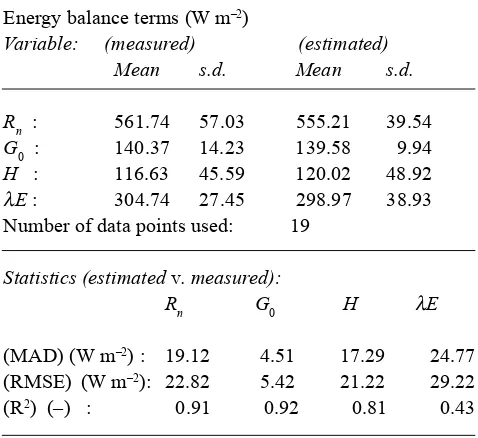
The four energy balance terms predicted versus the measured values are shown in Figure 1. Table 1 shows the predicted versus observed heat fluxes for the cotton dataset. Both mean and standard deviation of the predicted four energy balance terms compare very well with those measured.

At higher radiation levels, there is a tendency to underestimate R_n and G₀, whereas no obvious trends can be seen for H and λE (Fig.1). The underestimation for R_n and G₀ may be attributed to the temperature measurement procedure which may fail to catch the full diurnal effects of the shadows cast by the cotton plants on the bare soil between the rows.

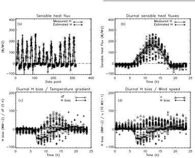
To investigate the behaviour of SEBS estimated sensible heat flux with respect to input variables and to explain the deviations, several plots are presented in Fig. 2; the bias between SEBS-estimated Hand measured His confined mostly to within around 30 W m–2_{, indicating good}

agreement with measured values. The biggest discrepancy occurs at data point 9 (9.55 h) at which the estimated sensible heat flux is 58.90 W m–2 _{more than the measured value. This}

situation corresponds to wind across the cotton row from the east (wind direction = 100 degrees), with very low wind speed (0.37 m s–1_{). Hence, when the wind speed is low, the}

uncertainty in the estimated flux terms becomes large. The reason for such uncertainty will be investigated with the help of two other field datasets that cover several complete diurnal cycles.

RESULTS FOR SHRUB DATA

For this dataset, Table 2 shows that both mean and standard deviation of SEBS estimated net radiation R_nand sensible heat flux H are in good agreement with measured values although SEBS overestimates the soil heat flux G₀ and underestimates the latent heat flux λE.

Obviously, due to the complexity of the underlying heterogeneous terrain and the difficulty in describing the vegetation cover for this dataset, the larger uncertainties in model parameters may cause greater discrepancies between estimates and observations than occurred with the cotton dataset.

To investigate the diurnal behaviour of SEBS estimated sensible heat flux with respect to input variables and to explain the deviations, several plots are presented in Fig. 3 which shows the dynamic behaviour of the estimated H follows that of measured H very well (Fig. 3a). The mean estimated H and the mean measured H compare very well Table 1. Statistics of SEBS estimated versus observed heat fluxes of the Cotton dataset

(s.d.: Standard deviation; MAD: Mean Absolute Deviation; RMSE: Root Mean Squared Error; R2_{: Coefficient of}

determination)

Energy balance terms (W m–2₎

Variable: (measured) (estimated)

Mean s.d. Mean s.d.

R_n : 561.74 57.03 555.21 39.54

G₀ : 140.37 14.23 139.58 9.94

H : 116.63 45.59 120.02 48.92

λE : 304.74 27.45 298.97 38.93

Number of data points used: 19

Statistics (estimated v. measured):

R_n G₀ H λE

(MAD) (W m–2_{) : 19.12 4.51 17.29 24.77}

(RMSE) (W m–2_{): 22.82 5.42 21.22 29.22}

Fig. 1. SEBS Estimated versus measured surface energy balance terms for cotton data

92

diurnally (Fig. 3b) although there are a few outliers in the afternoon and at night. The mean diurnal biases between SEBS estimated and measured H are within around 50 W m–2_{, indicating good agreement with measured values.}

The biggest biases of around 50 W m–2 _{occur from 7.00 to}

10.00 h (Fig. 3c) corresponding to the morning transition (the sun rises at approximately 6.30 h) from nightly stable condition to daily unstable condition, marked by the change of sign of the temperature gradient (surface temperature minus air temperature) from slightly negative to positive. Figures 3c and 3d show that this change of stability is coupled strongly with the temperature gradient but less so with wind speed. Judged by these behaviours, and noticing that the sensible heat flux has the same or bigger sensitivity to stability correction than to other terms, it might be concluded tentatively that the currently available stability corrections fail to describe the transition period adequately. This may also explain why most previous remote sensing algorithms deal with estimates of heat fluxes around noon and seldom mention application in the morning hours.

Fig. 3. Time series (a) and diurnal variations (b) of SEBS estimated and measured sensible heat flux and diurnal biases (SEBS estimated minus measured sensible heat flux) (c,d) versus environmental variables for shrub data (the solid lines are mean values, the vertical error bars are

mean value ± one standard deviation; both temperature gradient and wind speed are scaled)

Table 2. Statistics of SEBS estimated versus observed heat fluxes of the shrub dataset

(s.d.: Standard deviation; MAD: Mean Absolute Deviation; RMSE: Root Mean Squared Error; R2_{: Coefficient of}

determination)

Energy balance terms (W m–2₎

Variable: (measured) (estimated)

mean s.d. mean s.d.

R_n : 140.24 228.80 126.73 248.49

G₀ : 4.30 94.75 31.19 61.15

H : 41.52 79.06 34.70 72.64

λE : 94.35 69.14 60.84 130.87

Number of data points used: 320

Statistics (estimated v. measured):

R_n G₀ H λE

(MAD) (W m–2_{) : 28.64 41.46 18.99 73.39}

(RMSE) (W m–2_{) : 35.11 46.29 28.61 82.79}

RESULTS FOR GRASS DATA

Similarly for the grass dataset (Table 3), both mean and standard deviation of SEBS estimated net radiation R_nand sensible heat flux H are in good agreement with measured values but SEBS overestimates the soil heat flux G₀ and underestimates the latent heat flux λE.

The overall results are very similar to those of the shrub dataset, indicating that SEBS estimated the four energy balance terms with good accuracy. Due to the complexity of the underlying heterogeneous terrain and the difficulty in describing the vegetation cover for this dataset, the larger uncertainties in model parameters are likely to cause greater discrepancies between estimates and observations than are shown within the cotton dataset .

Similarly, an analysis for the diurnal trend of biases will be carried out for this dataset. Figure 4 shows the plots needed for this investigation. As with the shrub dataset, the dynamic behaviour of estimated H follows that of measured H very well (Fig. 4a). The mean estimated H and the mean measured Hcompare well diurnally (Fig. 4b). The mean diurnal biases between SEBS-estimated H and measured H are less than around 40 W m–2_{. The biggest biases of around}

Table 3. Statistics of SEBS estimated versus observed heat fluxes of the grass dataset

(s.d.: Standard deviation; MAD: Mean Absolute Deviation; RMSE: Root Mean Squared Error; R2_{: Coefficient of}

determination)

Energy balance terms (W m–2₎

Variable: (measured) (estimated)

mean s.d. mean s.d.

R_n : 162.42 244.43 133.88 261.08

G₀ : 5.02 83.75 26.56 51.80

H : 44.73 78.58 48.36 85.66

λE : 112.66 97.38 78.10 126.69

Number of data points used: 281

Statistics (estimated v. measured):

R_n G₀ H λE

(MAD) (W m–2_{) : 34.60 37.57 24.3 53.75}

(RMSE)(W m–2_{) : 41.26 42.95 36.19 61.34}

(R2₎

( )

−

Fig. 4. Time series (a) and diurnal variations (b) of SEBS estimated and measured sensible heat flux and diurnal biases (SEBS estimated minus measured sensible heat flux) (c,d) versus environmental variables for grass data (the solid lines are mean values, the vertical error bars are

94

40 W m–2 _{occur from 7.00 to 9.00 h (Fig. 4c) corresponding}

to the morning transition (the sun rises at approximately 6.30 h) from the nightly stable condition to the daily unstable condition. Figures 4c and 4d show that the change in stability in this case is also coupled with the temperature gradient but less so with wind speed. This confirms that, as for the shrub dataset, the currently available stability corrections fail to describe the transition period. However, in contrast to the shrub data, bigger biases are also observed at 18.00 and 19.00 h. This situation corresponds to the transition from unstable to stable condition and is also coupled to the temperature gradient but not so much to the wind.

RESULTS FOR EFEDA DATA

First of all, the primary inputs to SEBS are derived in the same way as Su et al. (1999) and Su and Jacobs (2001). These inputs include: remote sensing physical variables derived from the TMS data (albedo, surface temperature, and Normalized Difference Vegetation Index) and radiosonde and surface in-situ data (clear sky downward shortwave radiation, clear sky downward longwave radiation, PBL-height, surface pressure, PBL-averaged specific humidity, PBL-averaged potential temperature, PBL-averaged horizontal wind speed). Other derived variables are described in Su and Jacobs (2001). The relevant inputs for this study are given in Table 4.

The results of SEBS calculations are shown in Fig. 5. The corresponding histogram of the calculated evaporative fractions is shown in Fig. 6. The SEBS estimates of evaporative fractions lie between 0 and 1. In the Barrax area, there is a clear distinction between irrigated and non-irrigated crops, fallow and bare soils. Two clear peaks appear in the histogram, one around 0.25 (fallow) and a smaller one around 0.70 (irrigated crops). Furthermore, the

pivot-Table 4. Inputs for the application of SEBS to the TMS data

Surface temperature (o_{C) TMS derivative}

Surface albedo (–) TMS derivative

NDVI (–) TMS derivative

PBL Depth (M) 750

PBL pressure (Pa) 85986.1

PBL potential temperature (K) 300.15

PBL specific humidity (kG/kG) 0.0093

PBL wind speed (m s–1_{) 8.0}

Surface pressure (Pa) 94000.0

Downward long-wave radiation (W m–2_{) 372.0}

Surface short-wave radiation (W m–2_{) 860.0}

Fig. 5. Map of SEBS estimated evaporative fractions with the TMS data for the Barrax area on 29 June 1991.

(Legend: scaled between 0 = black and 1 = white)

29 June '91

0 10000 20000 30000 40000

0.06 0.11 0.17 0.22 0.27 0.33 0.38 0.43 0.49 0.54 0.59 0.64 0.70 0.75 0.80 0.86 0.91 0.96

Evaporative fraction with 0.01 interval

Count

Fig. 6. Histogram of SEBS estimated evaporative fractions with the TMS data for the Barrax area on 29 June 1991 (count refers to number of pixels falling in the same 0.01 incremental interval)

irrigated circular patterns and the corresponding evaporative fraction values are clearly identifiable from the map of evaporative fractions.

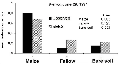
At three different surfaces in Barrax, simultaneous field measurements of heat flux densities were conducted during the EFEDA campaign: (1) irrigated maize, (2) fallow and (3) bare soil. Measurements at the maize and the fallow site were performed by the University of Karlsruhe, measurements at the bare soil site were made by CNRM Toulouse.

Table 5. Comparison SEBS estimates of evaporative fraction with field measurements in the Barrax area, 29 June 1991 (X,Y are image coordinates) (s.d. : standard deviation)

Site Data collection x Y Measured Estimated s.d. Estimated

Maize Karlsruhe 372 483 0.798 0.682 0.003

Fallow Karlsruhe 473 420 0.0984 0.266 0.125

Bare CNRM 367 462 0.154 0.218 0.027

Fig. 7. Comparison of SEBS estimates to field measurements of eva-porative fractions for three sites in the Barrax area on 29 June 1991

evaporative fractions obtained from field measurements and from SEBS for the three different surface types, together with the standard deviation of SEBS estimates determined using 3 × 3 pixels around the measurement masts. The actual values are given in Table 5, together with the standard deviation of the SEBS estimates.

The comparison of the SEBS estimates with field measurements is satisfactory but, due to the differences in measurement heights, the fetch areas of in-situ measurements and SEBS estimates may well differ which will contribute to the differences in the results. Further, since SEBS estimates are based on the instantaneous remotely sensed data while in-situ measurements are half-hourly averages, differences also occur due to the turbulent nature of the heat fluxes.

In this study it is not possible to investigate the quality of the input data due to lack of information. Although various studies have used the TMS data (Bastiaanssen, 1995; Su et al., 2000; Pelgrum, 2000) and the data should be of good quality in terms of calibration and corrections, some of the secondary variables were necessarily derived with rather limited knowledge of the surface conditions and of actual physical relationships.

ERROR ANALYSIS

Given a functional relationship of the form

{ }

y= (21)

the sensitivity of dependent variable y to a generic parameter or variable x in F{•} can de determined as

x x F y ⋅∆

∂ ∂ =

∆ (22)

To carry out an error analysis for the determination of the sensible heat flux H, Eqn. (5) is rewritten as follows,

(

)

or more simply

as t an r r

r H

+ +

= θ (24)

where θ =ρCp

(

)

    − = h an z d z ku r 0 0 * ln

1 _, 1

*

1 −

= kB

ku

r_t ,

            Ψ −       − Ψ − = L z L d z ku r h h h as 0 0 *

1 _{are the}

aerodynamic resistance at neutral stability, thermal dynamic resistance and resistance due to stability respectively.

96

Substitution of Eqn. (25) into Eqn. (22), yields the sensi-tivity of H to each term in Eqn. (24.).

Using the range of values from the cotton data, i.e. H= 50 ~ 200 (W m–2_{), u}

* =0.05 ~ 0.3 (MS-1), and (θ0 – θa) =5 ~ 20 (K), the sensitivity in Eqn. (24) to each term can also be applied to the primary terms, (θ0 – θa), u*, kB

–1_{, and Ψ}

h respectively. These sensitivities are given as:

∆H = 10•∆(θ

0 – θa), ∆H = 148•∆u*, ∆H = –25•∆kB–1,

∆H = –25•∆Ψ_h. Inserting typical values for the uncertainties

of the primary terms, the sensitivities are quantified as: 20, 11, –25 and –25 (W m–2_{), for ∆(θ}

0 – θa) = 2K, ∆u* = 25%,

∆kB–1 _{= 1, ∆Ψ}

h = 1, respectively. When the various terms are assumed independent of each other, the total uncertainty is around 40 (W m–2_{). Since in reality, at least some of the}

terms are correlated, the expected sensitivity can then be estimated in the order of 20 (W m–2_{), which is around 20%}

relative to the mean sensible heat flux H.

In a previous study, Su et al. (2001) have investigated the sensitivity of kB–1 _{to the physical and geometrical variables}

used in Eqn. (9) using a simpler version than Eqn. (9). By changing variable values as much as 50% with respect to reference values, they showed that the sensitivity of kB–1 _to

all parameters, except vegetation height, is comparable and the errors in the computed H are bounded by 37% relative to the mean measured H. The sensitivity of H to vegetation height approaches 46% of the mean measured H by far the largest. Since current SEBS formulation is superior to that used for the sensitivity analysis in Su et al. (2001) (the RMSE is 21.22 W m–2 _{in the present study, whereas it was}

27.29 W m-2_{), SEBS can give reliable estimates of H, as}

long as the variables used are accurate to within 50% of their actual values.

General remarks

After the derivation of sensible heat flux by solving Eqns. (4–6), the latent heat flux can be estimated as a residual by means of Eqn. (1), (e.g. Kalma and Jupp, 1990; Su, 2001). However, the uncertainty associated with the derived latent heat flux and consequently with the evaporative fraction is large, because the sensible heat flux is, under given surface conditions, determined solely by the surface temperature and the meteorological conditions at the reference height and is not constrained by the available energy. If the surface temperature or the meteorological variables have large uncertainties, the resultant latent heat flux and evaporative fraction will be affected. In the SEBS formulation, this uncertainty is limited by consideration of the energy balance at the limiting cases: the actual sensible heat flux H lies between the sensible heat flux at the wet limit H_wet derived from the combination equation, and the sensible heat flux

at the dry limit H_dry set by the available energy.

In this respect, SEBS is similar to previous algorithms that estimate relative evaporation by means of an index (e.g. the Crop Water Stress Index) using a combination equation (Jackson et al., 1981, 1988; Menenti and Choudhury, 1993; Moran et al., 1994; Pelgrum, 2000; Menenti et al., 2001). However, none of these algorithms incorporated the formulation of the roughness height for heat transfer explicitly; instead they used fixed values. Since the roughness height for heat transfer can vary with geometric and environmental variables by several orders of magnitude for different surface types, this can cause great uncertainties in estimation of heat fluxes or evaporation using radiometric temperature measurements (e.g. Verhoef et al., 1997; Massman, 1999a; Blümel, 1999; Su et al., 2001). Although it is possible to calibrate these algorithms such that their estimates reproduce observations at local scale, it would be very difficult to extrapolate them to regional/continental studies by means of satellite observations.

In Fig. 8, the sensible heat flux for the cotton dataset is estimated using a fixed value, kB–1 _{= 2.3, as is the practice}

in currently operational atmospheric models (e.g. van den Hurk et al., 2000). Compared to Fig. 2, the biases between estimated H and measured H reach 70 W m–2_{. Despite the}

fact that the value used for kB–1 _{= 2.3 is rather close to the}

estimated kB–1 _{= 2.85 (with a standard deviation of 0.49),}

neglecting the diurnal variations in kB–1 _{results in a larger}

uncertainty in estimated sensible heat flux, especially at high radiation levels. Hence, using such a formulation to estimate heat fluxes with surface radiometric temperature, the uncertainty will be very large. This undermines the usefulness of the surface radiometric temperatures that have been available routinely for more than 20 years (e.g. the NOAA/AVHRR data) and explains why such measurements have not been adopted in operational weather services. Another conclusion is that when currently implemented land surface schemes in atmospheric models are used to predict surface temperature, the deviation from actual satellite measurements will be very large. Therefore, it is suggested the value of the approach proposed in this study should be exploited so that the wealth of satellite observations can be used to obtain more accurate model simulations and predictions. SEBS can also be extended to estimate actual evaporation, soil water availability and drought stress of agricultural crops.

Conclusions

infrared frequency range, in combination with meteorological data from a proper reference height given by either in-situ measurements for application to a point, and radiosonde or meteorological forecasts for application at larger scales.

SEBS has been applied to four different data sets derived from radiometric and meteorological measurements. On the basis of these experimental validations, SEBS can be used to estimate turbulent heat fluxes at different scales with acceptable accuracy. Some specific conclusions are as follows:

z The mean error of SEBS estimates is expected to be around 20% relative to the mean sensible heat flux H, when the input geometrical and physical variables are reliable. For regional scale applications, SEBS can give reliable estimates of H, as long as the geometrical variables used are accurate to within 50% of their actual values and the physical variables are accurate to ∆(θ0 – θa) = 2K and ∆u* = 25%.

z The errors in estimated sensible heat flux H due to uncertainty in roughness height for heat transfer given by Eqns. (8–9), are bigger than or comparable to those due to uncertainties in temperatures, wind speed and stability corrections. The extended model of Su et al. (2001) proposed here (Eqn. 9) provides an operational solution for regional scale applications using remotely sensed data.

z Currently available stability corrections are inadequate in describing the transition from nightly stable to daily unstable conditions.

Finally, the application of SEBS does not require any a priori knowledge of the actual turbulent heat fluxes, indicating that SEBS is a credible and independent approach. Due to this property, SEBS results may be used to validate and initialise hydrological, atmospheric and ecological models that usually require proper partition of the sensible and latent heat flux at different scales. SEBS results may also be used via data assimilation in the above models to

Fig. 8. Same as Figure 2 for the cotton data, but estimated using a fixed value, _kB−1_{=2.3, as used in currently operational}

98

increase the reliability of the model simulations and predictions. Another approach would be to implement the representation of surface flux exchanges as described in SEBS into a Land Data Assimilation System (LDAS: see, for example, http://ldas.gsfc.nasa.gov/LDASnew/ index.html), then to assimilate the remotely-sensed data, including surface temperature, into the LDAS using modern data assimilation techniques. As evidenced by the presentations at the “International Workshop on Catchment-scale Hydrological Modelling and Data Assimilation, Wageningen, Sep. 3-5, 2001 (http://www.wau.nl/whh/ wrkshp/), advances in improving parameterisation and predictability of hydrological models, physically-based distributed models in particular, will rely heavily on the understanding of physical processes at different scales as well as the ability to obtain distributed physical information; satellite Earth observation will prove of paramount importance in the future.

Acknowledgements

This work was funded jointly by the Dutch Remote Sensing Board (BCRS), the Dutch Ministry of Agriculture, Nature Management and Fisheries (LNV), and the Royal Netherlands Academy of Science (KNAW). Constructive comments and assistance from Li Jia, Gerbert Roerink, Claire Jacobs, Jun Wen, Han Rauwerda (Alterra) and Bart van den Hurk (KNMI) are gratefully appreciated. The author is grateful to Bill Kustas (USDA/ARS) who kindly provided the three field data sets used in this study. The author is also grateful to the editor and three anonymous reviewers for their frank and constructive criticisms.

References

Bastiaanssen, W.G.M., 1998. Regionalization of surface flux densities and moisture indicators in composite terrain – A remote sensing approach under clear skies in Mediterranean climates. Ph.D. thesis, Wageningen Agricultural University, The Netherlands, 273 pp.

Beljaars, A.C.M. and Holtslag, A.A.M., 1991. Flux parameterization over land surfaces for atmospheric models, J. Appl. Meteorol., 30, 327–341.

Blümel, K., 1999. A simple formula for estimation of the roughness length for heat transfer over partly vegetated surfaces, J. Appl. Meteorol., 38, 814–829.

Bolle, H.-J., André, J.C., Arrue, J.L., Barth, H.K., Bessemoulin, P., Brasa, A., de Bruin, H.A.R., Cruces, J., Dugdale, G., Engman, E.T., Evans, D.L., Fantechi, R., Fiedler, F., van de Griend, A., Imeson, A.C., Jochum, A., Kabat, P., Kratzsch, T., Lagouarde, J.-P., Langer, I., Llamas, R., Lopez-Baeza, E., Melia Miralles, J., Muniosguren, L.S., Nerry, F., Noilhan, J., Oliver, H.R., Roth, R., Saatchi, S.S., Sanchez Diaz, J., de Santa Olalla, M., Shuttleworth, W.J., Sogaard, H., Stricker, H., Thornes, J.,

Vauclin, M. and Wickland, D., 1993. EFEDA: European field experiments in a desertification-threatened area. Ann. Geophys.,

11,173–189.

Bosveld, F.C., 1999. Exchange processes between a coniferous forest and the atmosphere. Ph.D. dissertation, Wageningen University, 181pp.

Bowen, I.S., 1926. The ratio of heat losses by conduction and by evaporation from any water surface. Phys. Rev., 27, 779–787. Brutsaert, W., 1982. Evaporation into the atmosphere. D. Reidel,

299pp.

Brutsaert, W., 1999. Aspects of bulk atmospheric boundary layer similarity under free-convective conditions. Rev. Geophy., 37, 439–451.

Campbell, G.S. and Norman, J.M., 1998. An introduction to environmental biophysics. Springer, 286pp.

Choudhury, B.J., Reginato, R.J. and Idso, S.B., 1986. An analysis of infrared temperature observations over wheat and calculation of latent heat flux. Agr. Forest Meteorol., 37, 75–88.

Choudhury, B.J. and Monteith, J.L., 1988. A four layer model for the heat budget of homogeneous land surfaces. Quart. J. Roy. Meteorol. Soc., 114, 373–398.

Famiglietti, J.S. and Wood, E.F., 1994. Multiscale modeling of spatially variable water and energy balance processes. Water. Resour. Res., 30, 3061–3078.

Humes, K.S., Kustas, W.P., Moran, M.S., Nichols, W.D. and Weltz, M.A., 1994. Variability of emissivity and surface temperature over a sparsely vegetated surface. Water Resour. Res., 30, 1299– 1310.

Jackson, R.D., Idso, S.B., Reginato, R.J. and Pinter Jr., P.J., 1981. Canopy temperature as a crop water stress indicator. Water Resour. Res., 17, 1133–1138.

Jackson, R.D., Kustas, W.P. and Choudhury, B.J., 1988. A re-examination of the crop water stress index. Irrig. Sci., 9, 309– 317.

Kalma, J.D. and Jupp, D.L.B., 1990. Estimating evaporation from pasture using infrared thermometry: evaluation of a one-layer resistance model. Agr. Forest Meteorol., 51, 223–246. Katul, G.G. and Parlange, M.B., 1992. A Penman-Brutsaert model

for wet surface evaporation. Water Resour. Res., 28, 121–126. Kustas, W.P. and Norman, J.M., 1996. Use of remote sensing for evapotranspiration monitoring over land surfaces. Hydrol. Sci. J., 41, 495–516.

Kustas, W. P. and Norman, J.M., 1999. Evaluation of soil and vegetation heat flux predictions using a simple two-source model with radiometric temperatures for partial canopy cover. Agr. Forest. Meteorol., 94,13–29.

Kustas, W.P., 1990. Estimates of evapotranspiration with a one and two layer model of heat transfer over partial canopy layer.

J. Appl. Meteorol., 29, 704–715.

Kustas, W.P. and Daughtry, C.S.T., 1989. Estimation of the soil heat flux/net radiation ratio from spectral data. Agr. Forest. Meteorol., 49, 205–223.

Kustas, W.P. and Goodrich, D.C., 1994, Preface. Water Resour. Res., 30, 1211–1225.

Kustas, W.P., Choudhury, B.J., Kunkel, K.E. and Gay, L.W., 1989a. Estimate of the aerodynamic roughness parameters over an incomplete canopy cover of cotton. Agric. Forest. Meteorol.,

46, 91–105.

Kustas, W.P., Choudhury, B.J., Inoue, Y., Pinter, P.J., Moran, M.S., Jackson, R.D. and Reginato, R.J., 1989b. Ground and aircraft infrared observations over a partially-vegetated area. Int. J. Remote Sens., 11, 409–427.

Kustas, W.P., Moran, M.S., Humes, K.S., Stannard, D.I., Pinter Jr., P.J., Hipps, L.E., Swiatek, E. and Goodrich, D.C., 1994b. Surface energy balance estimates at local and regional scales using optical remote sensing from an aircraft platform and atmospheric data collected over semiarid rangelands. Water Resour. Res., 30, 1241–1259.

Li, Z.-L., Stoll, M.P., Zhang, R., Jia, L. and Su, Z., 2000. On the separate retrieval of soil and vegetation temperatures from ATSR data. Sci. in China, series E, 30, 27–38.

Massman, W.J., 1997. An analytical one-dimensional model of momentum transfer by vegetation of arbitrary structure. Bound-Lay. Meteorol., 83, 407–421.

Massman, W.J., 1999a. A model study of −1

H

kB for vegetated surfaces using ‘localized near-field’ Lagrangian theory. J. Hydrol., 223, 27–43.

Massman, W.J., 1999b. Molecular diffusivities of Hg vapor in air, O₂ and N₂ near STP and the kinematic viscosity and the thermal diffusivity of air near STP. Atmos. Environ., 33, 453– 457.

Menenti, M., 1984. Physical aspects of and determination of evaporation in deserts applying remote sensing techniques. Report 10 (special issue), Institute for Land and Water Management Research (ICW), The Netherlands, 202pp. Menenti, M. and Choudhury, B.J., 1993. Parametrization of land

surface evapotranspiration using a location-dependent potential evapotranspiration and surface temperature range. In: Exchange processes at the land surface for a range of space and time scales, Bolle, H.J. et al. (Eds.). IAHS Publ. no. 212: 561–568. Menenti, M., Choudhury, B.J. and Di Girolamo, N., 2001. Monitoring of actual evaporation in the Aral Basin using AVHRR observations and 4DDA results. In: Advanced Earth Observation – Land Surface Climate, Z. Su and C. Jacobs (Eds.). Report USP-2, 01-02, Publications of the National Remote Sensing Board (BCRS), 79–83.

Monteith, J.L., 1965. Evaporation and environment. Sym. Soc. Exp. Biol., 19, 205–234.

Monteith, J.L., 1973. Principles of environmental physics. Edward Arnold Press. 241 pp.

Moran, M.S., Clarke, T.R., Inoue, Y. and Vidal, A., 1994. Estimating crop water deficit using the relation between surface-air temperature and spectral vegetation index. Remote Sens. Environ., 49, 246–263.

Morton, F.I., 1983. Operational estimates of areal evapo-transpiration and their significance to the practice of hydrology.

J. Hydrol., 66, 1–76.

Norman, J. M., Kustas, W. P. and Humes, K.S., 1995. A two-source approach for estimating soil and vegetation energy fluxes from observations of directional radiometric surface temperature. Agr. Forest. Meteorol., 77, 263–293.

Pelgrum, H., 2000. Spatial aggregation of land surface characteristics – impact of resolution of remote sensing data on land surface modelling. Ph.D. thesis, Wageningen University. 151 pp.

Penman, H.L., 1948. Natural evaporation from open water, bare soil and grass. Proc. Roy. Soc., A, 193, 120–146.

Press, W.H., Teukolsky, S.A., Vetterling, W.T. and Flannery, B.P., 1997. Numerical Recipes in C: The Art of Scientific Computing. Cambridge Univ. Press. 994pp.

Priestly, C.H.B. and Taylor, R.J., 1972. On the assessment of surface heat flux and evaporation using large-scale parameters.

Mon. Weather Rev., 100, 81–92.

Sellers, P.J., Randall, D.A., Collatz, G.J., Berry, J.A., Field, C.B., Dazlich, D.A., Zhang, C., Collelo, G.D. and Nounoua, L., 1996. A revised land surface parameterisation (SiB2) for atmospheric GCMS, part 1: model formulation. J. Climate, 9, 676–705. Stull, R.B., 1988. An introduction to boundary layer meteorology.

Kluwer Academic Publ. 670pp.

Su, Z., 2000. Remote sensing of land use and vegetation for mesoscale hydrological studies. Int. J. Remote Sens., 21, 213– 233.

Su, Z., 2001. A Surface Energy Balance System (SEBS) for estimation of turbulent heat fluxes from point to continental scale, In: Advanced Earth Observation – Land Surface Climate,

Z. Su and Jacobs, C. (Eds.). Publications of the National Remote Sensing Board (BCRS), USP-2, 01-02. 184pp.

Su, Z. and Jacobs, C. (Eds.), 2001. Advanced Earth Observation – Land Surface Climate. Report USP-2, 01-02, Publications of the National Remote Sensing Board (BCRS). 184pp.

Su, Z. and Menenti, M. (Eds.), 1999. Mesoscale climate hydrology: the contribution of the new observing systems. Report USP-2, 99-05, Publications of the National Remote Sensing Board (BCRS). 141pp.

Su, Z., Pelgrum, H. and Menenti, M., 1999. Aggregation effects of surface heterogeneity in land surface processes. Hydrol. Earth Syst. Sci., 3, 549–563.

Su, Z., Menenti, M., Pelgrum, H., van den Hurk, B.J.J.M. and Bastiaanssen, W.G.M., 1998. Remote sensing of land surface fluxes for updating numerical weather predictions. In:

Operational Remote Sensing for Sustainable Development,

G.J.A. Nieuwenhuis, R.A. Vaughan and M. Molenaar (Eds.). Balkema, The Netherlands. 393–402.

Su, Z., Schmugge, T., Kustas, W.P. and Massman, W.J., 2001. An evaluation of two models for estimation of the roughness height for heat transfer between the land surface and the atmosphere.

J. Appl. Meteorol. 40, 1933–1951.

van den Hurk, B.J.J.M. and Holtslag, A.A.M., 1995. On the bulk parameterization of surface fluxes for various conditions and parameter ranges. Bound-Lay. Meteorol., 82, 199–234. van den Hurk, B.J.J.M., Viterbo, P., Beljaars, A.C.M. and Betts,

A.K., 2000. Offline validation of the ERA40 surface scheme. ECMWF TechMemo 295.

Verhoef, A., de Bruin, H.A.R. and van den Hurk, B.J.J.M., 1997. Some practical notes on the parameter for sparse vegetation J. Appl. Meteorol., 36, 560–572.

Weltz, M.A., Ritchie, J.C. and Fox, H.D., 1994. Comparison of laser and field measurements of vegetation height and canopy cover. Water Resour. Res., 30, 1311–1319.

Wieringa, J., 1986. Roughness-dependent geographical interpolation of surface wind speed averages. Quart. J. Roy. Meteorol. Soc., 112, 867–889.

Wieringa, J., 1993. Representative roughness parameters for homogeneous terrain. Bound-Lay. Meteorol., 63,323–363. Zhan, X., Kustas, W.P. and Humes, K.S., 1996. An intercomparison