Subgrid spatial variability of soil hydraulic functions for hydrological modelling

www.hydrol-earth-syst-sci.net/20/2557/2016/ doi:10.5194/hess-20-2557-2016

© Author(s) 2016. CC Attribution 3.0 License.

Subgrid spatial variability of soil hydraulic functions

for hydrological modelling

Phillip Kreye and Günter Meon

Department of Hydrology, Water Resources Management and Water Protection, Leichtweiß-Institute for Hydraulic Engineering and Water Resources, University of Braunschweig, Beethovenstr. 51a, 38106 Braunschweig, Germany Correspondence to:Phillip Kreye ([email protected])

Received: 29 January 2016 – Published in Hydrol. Earth Syst. Sci. Discuss.: 18 February 2016 Revised: 6 June 2016 – Accepted: 13 June 2016 – Published: 1 July 2016

Abstract. State-of-the-art hydrological applications require a process-based, spatially distributed hydrological model. Runoff characteristics are demanded to be well reproduced by the model. Despite that, the model should be able to de-scribe the processes at a subcatchment scale in a physically credible way. The objective of this study is to present a ro-bust procedure to generate various sets of parameterisations of soil hydraulic functions for the description of soil het-erogeneity on a subgrid scale. Relations between Rosetta-generated values of saturated hydraulic conductivity (Ks) and

van Genuchten’s parameters of soil hydraulic functions were statistically analysed. An universal function that is valid for the complete bandwidth of Ks values could not be found.

After concentrating on natural texture classes, strong corlations were identified for all parameters. The obtained re-gression results were used to parameterise sets of hydraulic functions for each soil class. The methodology presented in this study is applicable on a wide range of spatial scales and does not need input data from field studies. The develop-ments were implemented into a hydrological modelling sys-tem.

1 Introduction

One of the major challenges in hydrological process mod-elling is to minimise the discrepancy between model and data scale as described e.g. by Blöschl and Sivapalan (1995) or Hopmans et al. (2002).

State-of-the-art hydrological applications require a process-based, spatially distributed hydrological model. As the first objective, runoff characteristics are demanded to be

well reproduced by the model. Despite that, and even for large-scale applications, the model should be able to describe the processes at a subcatchment scale in a physically credible way. Following Blöschl and Sivapalan (1995), hydrological processes that are dominant at spatial scales larger than the smallest calculation unit (hydrological response unit respective elementary grid size) of the model are assumed to be described directly by the model. Small-scale processes below the smallest spatial calculation unit are assumed to be described indirectly by the model, e.g. by calibration.

The simulation of soil water movements and storages can be particularly sensitive with respect to many model outputs (total runoff, infiltration, groundwater recharge, actual evap-otranspiration, etc.). Especially the water content of the soil near the surface is a decisive factor for the runoff genera-tion (e.g. Binley et al., 1989a; Beven, 1995; de Roo et al., 1996; Coles et al., 1997; Bronstert and Bárdossy, 1999; Entin et al., 2000; Hasenauer et al., 2009). Further, the parameteri-sation of field-saturated hydraulic conductivities (Ks values,

e.g. cm day−1) with proxy data is an essential factor for many physically based hydrological models (Gupta et al., 2006).

be physically based; instead, the question is how they should be based on physics”.

Area-wide measured data of basic soil properties or even of soil hydraulic properties are not available for most hy-drological model applications at the meso- and macroscale. However, in many cases rough information about the soil (e.g. soil maps) is available on a very coarse spatial resolu-tion (1 : 50 000 at best). Using such rough input data does not allow direct parameterisation of any subgrid variability. In addition, soil maps are already products of regionalised input data. Consequentially, all soil hydraulic parameters based on soil maps can be interpreted (only) as effective parameters.

In this study, the subgrid spatial variability for the param-eterisation of soil hydraulic functions will be derived indi-rectly from soil map information. To achieve this, three state-ments are formulated and will be discussed below:

1. The spatial variability of saturated hydraulic conductiv-ity of soils on a subgrid scale can be expressed by a lognormal distribution.

2. There are relationships between the saturated hydraulic conductivity and the parameters of soil hydraulic func-tions.

3. These relationships are mirrored in the parameters gen-erated by the software Rosetta (Schaap et al., 2001). They can be used to simulate a subgrid spatial variabil-ity in a straightforward procedure, which does not re-quire measured samples of soil properties.

The first statement was widely acknowledged in numerous studies (e.g. Law, 1944; Baker and Bouma, 1976; Sharma et al., 1980; Lauren et al., 1988; Binley et al., 1989b; Goodrich, 1990; Vauclin et al., 1994; Mallants et al., 1997; Bosch and West, 1998; Viera et al., 2011, and many more). The second statement was investigated in several studies as well. However, compared to the first statement, the avail-able studies are less clear. Carsel and Parrish (1988) used approx. 3000 measurements of soil textures and bulk den-sities, which were summarised into 12 major texture classes. They approximated van Genuchten (1980) parameters (VGP)

2S, 2R, α and n as well as Ks values utilising the

em-pirical regression functions of Rawls et al. (1993) to de-scribe soil hydraulic functions. In a following step, Gaussian distributions for the VGP were approximated by using the Johnson system of transformations. This was done for every VGP independently. After the transformation, high correla-tions were found between VGP andKs values. In a

follow-ing study, de Rooij et al. (2004) used approx. 140 samples from two layers of an agricultural soil to fit VGP and Ks

values each. Relationships between the VGP and theKs

val-ues were found by means of regression analyses. However, these relationships were considered to be too weak for us-ing the Ks values as a direct predictor for the VGP. In the

next step, they used these relationships as additional infor-mation for estimating probability distribution functions for

each VGP. The assumption ofKsbeing lognormal distributed

was considered as well. In a study of Li et al. (2007), data were measured experimentally to describe 63pF curves as well as correspondingKs values, texture information, bulk

densities and fractions of organic matter.pF is defined as log₁₀ values of the absolute soil pressure heads. The model of van Genuchten (1980) was adapted to fit the measured data in order to obtain pF curves. This research found high correlations between VGP, measured texture classes and bulk density as well as weak correlations between mea-suredKs values and bulk densities. No significant

correla-tions were found betweenKsand the texture of the soil.

Re-gression analyses were not conducted forKsand VGP.

How-ever, the other regressions of Li et al. (2007) indicate that there seems to be no significant relationship. Botros et al. (2009) carried out measurements to obtainpF curves for nearly 100 sediment cores. They analysed the dependence among measuredKsvalues and VGP, which were fitted to the

measured pairs of the soil water content (2) and the soil pres-sure head (h). Significant correlations were found between

Ks andα,nand2S;Ks and2R were also correlated, but

did not yield significance. A factor all these studies have in common is that any analysis is always based on measured in-put data of soil properties. Aside from that, rather elaborate numerical simulations were necessary in many cases. As a general note, relationships between the VGP andKs values

were found in many studies.

Besides the lack of measured soil samples, the effort of parameterisation by means of sophisticated procedures that often require Monte Carlo applications is very high even for models operating on the hill slope scale. This effort is much higher for large areas and huge timescales as it is usual in e.g. climate change hydrological modelling. Consequently, the use of effective parameter sets and powerful calibration procedures is widespread. On the other hand, some kind of calibration parameters are always needed in hydrologi-cal modelling. Based on this, the third (innovative) statement was formulated. Premised on profound analyses of the rela-tionship between Rosetta-generatedKs values and VGP for

several texture classes, the objective of this study is to con-sider the subgrid spatial variability of soil hydraulic functions for hydrological modelling by using these relationships. It is worth mentioning that the methodology presented in this study is applicable for a wide range of spatial scales and does not need measured input data from field studies.

2 Methodology

In this section, we shortly give the required theoretical back-ground in soil physics and statistics. Further, the creation of a database is presented by means of the software Rosetta. The database contains the parameters and Ks values for

theKsvalues and the parameters of the soil hydraulic

func-tions of the generated databases are analysed. 2.1 Soil hydraulic functions

Since the objective of this paper is the consideration of sub-grid variability of the parameterisation of soil hydraulic func-tions at the meso- and macroscale, the model for the de-scription of the soil hydraulic functions has to be deter-mined in the first place. The use of proxy information is one of very few possibilities to parameterise soil hydraulic functions extensively for large hydrological model areas. As the software Rosetta will be used for this application (see Sect. 2.2), the obtained parameters are limited to the model of van Genuchten (1980). However, this model is widely used in hydrological and soil physical disciplines for describing the relation between water content and pressure head in soils:

2(h)=2R+(2S−2R)1+(α|h|)n −m

. (1)

There are synonymic designations for the relationship be-tween water content and pressure head; see Durner and Flüh-ler (2006) for details. In this study, the designationpF curve is used. In Eq. (1),2(h)denotes the volumetric water con-tent (cm3cm−3),h(cm) marks the pressure head of the soil,

2Rand2S(cm3cm−3) are defined as the residual and

sat-urated water contents of the soil, whereas α (cm−1) n(–) and m(–) are shape parameters of the model. Both shape parameters have a weak physical interpretation. The inverse ofα(and alson) is slightly related to the air entry pressure head (however, Eq. (1) has no defined air entry value). The parametern is connected to the width of the pore size dis-tribution of the soil between2Sand air entry pressure head.

The product mnis related to the width of the pore size dis-tribution of the soil between air entry pressure head and2R

(Durner and Flühler, 2006; Peters and Durner, 2006). Studies of Wösten and van Genuchten (1988) and van Genuchten and Nielsen (1985) analysed the influence of these parameters on the shape of the modelledpF curve in detail. The parame-termis in most cases approximated as 1−1

n, which reduces the flexibility of the model, but enables a closed form expres-sion for the unsaturated hydraulic conductivity by combining Eq. (1) with the pore size model of Mualem (1976):

K(2)=KsSel

h 1−

1−S_e(m−1)

mi2

, (2)

with the effective saturationSe(cm3cm−3) as

Se=

2−2r

2s−2r

. (3)

In general, the absolute values of Eq. (2) are scaled by the saturated hydraulic conductivityKs(cm day−1). The

param-eter l(–) can be approximated as 0.5 (Kutílek and Nielsen, 1994; Hillel, 1998). The unsaturated hydraulic conductivity (K(2)respectivelyK(h)) can either be formulated in depen-dency of the soil water content2as shown in Eq. (2), or of the pressure headh.

Table 1.Definitions of the used texture classes. The fractions of sand, silt and clay is processed out of the soil map for Lower Sax-ony (Boess et al., 2004) and the German soil classification system (Sponagel, 2005).

Abbreviation Definition Sand Silt Clay

(%) (%) (%)

Lt Clayey loam 25 40 35

Lu Silty loam 18.5 58 23.5

Ls Sandy loam 44 35 21

Ut Clayey silt 9 74 17

Ul Loamy silt 27 58 15

Us Sandy silt 32.5 65 2.5

Sl Loamy sand 65 25 10

Su Silty sand 63.5 32.5 4

S Sand 85 10 5

Ss Pure sand 92.5 5 2.5

2.2 Parameters for soil hydraulic functions

One objective is to investigate for correlations between Rosetta-generated VGP and Ks values. To formulate

sta-tistically significant statements, a representative population for the statistical analyses has to be considered. Therefore, a short algorithm was developed to create trios of numbers within a range of 0–100. These trios were randomly gener-ated with the precondition that the sum of each trio has to be 100. The numbers of each trio are assigned to be a per-centage fraction of sand, silt and clay. A total of 106 ficti-tious samples of possible compositions of texture fractions were obtained in this manner. All three texture fractions are characterised by the same distribution with an expected value of 33.3 % sand/silt/clay. The large number of generated sam-ples was empirically determined in order to get a represen-tative population for the statistical analyses. The regression results were stable for populations≥105. The number was increased to 106to safeguard validity.

The free-of-charge software Rosetta (Schaap et al., 2001) was utilised to estimate the VGP2R,2S,αandnas well

as Ks values per sample. It is based on neural network

analyses and was calibrated by means of a large database comprised of 2134 soil samples that consists of more than 20 000 pairs of2andhin total. For the saturated hydraulic conductivity, 1306 soil samples were available. A total of 235 samples also contained data for the unsaturated hy-draulic conductivity function K(2) respectively K(h) in-cluding more than 4000 data points (Schaap et al., 1998, 2001). The database UNSODA (Leij et al., 1996; Nemes et al., 2001) contributes significantly to these data points. Ad-ditional information about early neural network applications for parameterisation of soil hydraulic functions can also be found in Schaap and Bouten (1996).

The VGP sets (includingKsvalues), obtained with Rosetta

are hereafter called database 0. In addition to this database, gradual reductions of database 0 were carried out. These reductions were a result of the evaluation of the regres-sion analyses. Further reasons of the reduction are given in Sect. 3. At total four different databases were generated (database 0 and three derivatives of database 0):

1. The complete database 0, which consists of the total of 106VGP sets includingKsvalues.

2. A reduced database 1 based on the condition that

Ks<150 cm day−1. Approx. 95 % of the parameter sets

of database 0 are still included.

3. A reduced database 2 based on the condition that

Ks<150 cm day−1 and2R<9 %. Approx. 70.5 % of

the parameter sets of database 0 are still included. 4. Several selected databases 3x: Variant A: subdivision

based on natural texture classes according to the soil map of Lower Saxony, Germany. Variant B: subdivision based on soil hydraulic properties.

2.2.1 Generation of databases 3x, variant A:

classification by soil map

The final reductions to databases 3xwere conducted for two reasons: firstly, it is suspected that many grain size compo-sitions in database 0 are unrealistic (e.g. 100 % clay or 50 % clay and 50 % sand) causing the neural network of Rosetta to extrapolate the parameters for these compositions. This may have noisy effects on possible correlations betweenKs

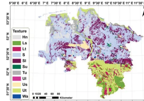
and the VGP. Secondly, the presented approach is tailored to hydrological modelling at the meso- and macroscale with-out employing measured data. In most cases only rough in-formation about the soil (e.g. soil maps) is available for the model area. For that reason, the database was further reduced to obtain natural texture classes, which can be found in many soil maps. Suitable soil maps (or similar products) are widely available around the world. We used the German soil map of Lower Saxony (Boess et al., 2004); see Fig. 1. Out of this, common natural compositions of grain sizes were iso-lated from the data sets of database 0 in order to generate databases 3x(variant A). Abbreviations of the texture classes are defined in Table 1 and were assigned according to the German soil classification system (Sponagel, 2005). A pre-defined texture class for boggy soils (Hn) is not available. Silty clay (Tu) has similar properties as clayey loam (Lt), therefore these two texture classes (Hn, Tu) are not included in the following analyses. Instead, the texture classes for silty loam (Lu) and pure sand (Ss) were added. These tex-ture classes are not shown in the soil map (Fig. 1). However, both are contained in other soil maps of Germany. Around each texture fraction, a±5 % boundary in each direction was considered in order to get a representative number of van Genuchten data sets for the regression analyses. Note that in total more than 105parameter sets of database 0 are still

Figure 1.Soil map of Lower Saxony, Germany (Boess et al., 2004). Ls is sandy loam, Lt is clayey loam, S is sand, Sl is loamy sand, Su is silty sand, Tu is silty clay, Ul is loamy silt, Us is sandy silt, Ut is clayey silt; see Table 1. In addition, Hn stands for boggy soils and Wa stands for water bodies (lakes, rivers).

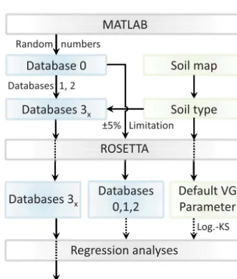
included in the databases 3x (variant A). The procedure to obtain the VGP andKsvalues is graphically shown in Fig. 3.

2.2.2 Generation of databases 3x, variant B:

classification by cluster analyses

Twarakavi et al. (2010) introduced a procedure to classify soils based on their hydraulic properties. To achieve this, they used the k-means clustering algorithm. The same al-gorithm was used in this study to subdivide database 0 by means of hydraulic properties. This algorithm is available in MATLAB. We standardised the VGP to avoid scale effects that influence the weightings in a negative way. Minimisa-tion of euclidean distance was applied as objective funcMinimisa-tion. The number of resulting subdivisions (classes) is freely ad-justable. We used 255 different target classes, starting with 2 and going up to 5680 classes.

2.3 Regression analyses for soil hydraulic parameters A flexible exponential regression model is used, since the modalities of the relations between theKs values and the

VGP are unknown:

f (x)=aebx+cedx, (4)

where a, b, c and d (–) are fitting parameters and e (–) is Euler’s number. The model is adjusted by means of the Levenberg–Marquardt algorithm (Marquardt, 1963).

where the matrixYdenotes the dependent variables, which are assumed to be correlated among themselves. The matrix Xincludes the independent variables, the matrixBcomprises the fitting coefficients and Egives the matrix of residuals. The indexndenotes the number of samples,dthe number of subjects andpthe number of predictor variables.

To evaluate the quality of the regressions, the coefficient of determinationR2is calculated as follows (Sachs, 2004):

R2=SSY−RSS

SSY =

MSS SSY =1−

RSS SSY

=1−

n P

i=1

yi− ˆyi 2

n P

i=1

(yi−y)2

, (6)

with

y=1 k

k X

i=1

yi. (7)

SSY is the total, RSS is the residual and MSS is the regres-sion sum of squares. By standardisation of MSS with SSY, the coefficient of determination R2 is obtained.yi denotes a data value andy describes the average of all data values, whereas yˆi symbolises a computed value of the regression model.R2ranges from 0 (no relation) to 1 (perfect fit).

For consideration of nonlinearities, Spearman’s rank cor-relation coefficientrspearcan be calculated in addition to the

coefficient of determination (Sachs, 2004):

rspear=1−

6 k P

i=1

(rg (xi)−rg (yi))2

k(k−1)2 . (8)

The values rg(xi) and rg(yi), which are sorted into ranks (rg), are the values of the data set and the fitted model with the total number ofk.rspear has a range from−1 to 1,

whereby 0 denotes no correlation and 1/−1 describe a perfect positive/negative correlation, respectively.

3 Results and discussion 3.1 Regression analyses

3.1.1 Complete database 0 and reduced databases 1 and 2

Regression analyses based on Eq. (4) were performed for the database 0 and for each of the reduced databases 1 and 2.

TheKsvalues in relation to the2Rvalues resulted in low

correlations withR2of 0.43. A more structuredKs−2R

re-lation seems to arise forKsvalues smaller than 150 cm day−1

and 2R smaller than 9 %. Consequently, database 0 was

reduced to database 2 and R2 of the regression function,

which was computed out of the complete database 0, in-creased to 0.72. However, to obtain a function on the basis of database 2, new regression analyses were conducted leading toR2of 0.74. This function is shown in the first plot of Fig. 5. A similar approach was applied to evaluateKs and2S; no

significant correlations were obtained. Because of the high correlations found forKs−2Rin database 2, the reduction

of the database 0 was also applied for2S. However, only the

range of theKsvalues was reduced, leading to database 1. In

contrast toKs−2R, no significant correlations were found

betweenKs and2S based on the reduced database; see the

second plot of Fig. 5. Low correlations (R2=0.41) were found for the parameternwhen using database 0. An even lower fit (R2=0.25) was obtained when reducing database 0 to database 1 as seen in the third plot of Fig. 5. The analysis ofKsvs.αshows neither correlations for database 0 nor for

database 1 (fourth plot of Fig. 5).

Generally, in some sections of the scatter diagrams there seem to be more connections between theKsvalues and

pa-rameters of the soil hydraulic functions than in other sec-tions. However, these connections are very low and too un-certain for hydrological modelling purposes. A reduction of database 0 to database 1 respectively database 2 had a posi-tive effect on the regression of2Ronly. Apparently, it is not

possible to obtain four single regression functions, one for each parameter.

3.1.2 Databases 3x, variant A: classification by soil map

Univariate regression analyses

Regression analyses based on Eq. (4) were performed for each of the natural texture classes. Concerning2R, very high

R2 between 0.88 and 0.99 were found for 7 out of the 10 texture classes with an averageR2 of 0.96. The other three classes reached correlations withR2lower than 0.5; there-fore, these classes were not included in following analyses and applications. Generally, curves with aR2lower than 0.5 are not illustrated in the figures and tables. The regression curves of 2R are exponentially decreasing proportional to

decreasingKs values, which physically makes sense.

How-ever, we have to keep in mind that van Genuchten’s2Rhas

no clear physical interpretation and other fitting models for the pF curve actually have no residual water content (see e.g. Rossi and Nimmo, 1994). The high correlations between

2RandKsmay have to be considered as a kind of black box

correlation that is valid for the Rosetta-fed van Genuchten model only.

Concerning 2S, high R2 between 0.68 and 0.93 were

ef-fect on the slopes of the fitted regression models. Group one shows decreasing values of 2S with increasingKs values,

group two behaves the other way round. Assuming higher sand fractions causing higherKsvalues, the grain size

com-positions of group one are shifted in the direction to the centre of the texture triangle. This may cause smaller val-ues of2S. On the other hand, moving away from the centre

of the texture triangle with higher fractions of sand (as for group two) may have the opposite effect of increasing poros-ity. Both effects are imaginable, however, we do not want to overinterpret the physical impact of van Genuchten’s2S.

Concerningα, highR2values between 0.67 and 0.96 were found for four texture classes with an average R2 of 0.75. As given in Sect. 2.1, the parameter αis weakly related to the inverse of the air entry suction (not to forget that van Genuchten curves have no defined air entry value). In gen-eral, without focusing on van Genuchten’s model, the entry suction should be higher for fine-grained than for coarse-grained soils. This means that the entry suction should rather decrease with increasing Ks than increase. This connection

cannot be found for the texture class Lu. That is why this regression (Lu) is not considered in the subsequent analysis. Concerningn, very highR2between 0.63 and 1.00 were found for seven texture classes with an averageR2of 0.85. Especially for the two sandy texture classes, highly accurate fits were obtained. Under the assumption ofnbeing related to the pore size distribution, many different pore sizes lead to low values ofn, whereas many pores with a similar size lead to high values of n. In general, soils that are located near the borders of the texture triangle tend to have a more nar-row pore size distribution than soils located in the middle of the triangle. Taking into account that these soils (pure sand, pure silt) may have higher Ks values compared to loamy

soils, increasing Ks may be related to increasing values of

van Genuchten’sn. Again, we have to be careful not to over-stretch connections of Rosetta-generated VGP to measurable physical properties of soils.

All statistical quality values from the univariate regression analyses are listed in Table 2. Additionally,pvalues are in-cluded. Lowpvalues indicate a correlation betweenKsand

the parameters of the soil hydraulic functions. Allpvalues of Table 2 are nearly 0, yielding that all shown correlations are significant. Further, the square ofrspearyields approximately

R2 for most cases. This seems to validate R2 as a quality criterion for the regression analyses.

Multivariate regression analyses

Regression analyses based on Eq. (5) were performed for each of the natural texture classes. We used log₁₀(Ks) to

fill the matrix X. The matrix Y comprises2R,2S,n and

α. These more elaborate procedures, which consider the cor-relations among the dependent variables, serve as references for the previous results.

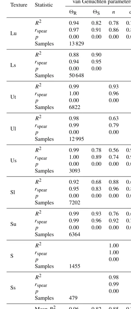
Table 2. Obtained coefficients of determination (R2), Spearman correlation (rspear) and belongingpvalue (p) as well as the sample size (Samples) for the regressions between theKs values and the soil hydraulic parameters for each texture class. Lu is silty loam, Ls is sandy loam, Ut is clayey silt, Ul is loamy silt, Us is sandy silt, Sl is loamy sand, Su is silty sand, S is sand, Ss is pure sand.

Texture Statistic van Genuchten parameters

2R 2S n α

Lu

R2 0.94 0.82 0.78 0.73

rspear 0.97 0.91 0.86 0.88

p 0.00 0.00 0.00 0.00

Samples 13 829

Ls

R2 0.88 0.90

rspear 0.94 0.95

p 0.00 0.00

Samples 50 648

Ut

R2 0.99 0.93

rspear 1.00 0.96

p 0.00 0.00

Samples 6822

Ul

R2 0.98 0.63

rspear 0.99 0.79

p 0.00 0.00

Samples 12 995

Us

R2 0.99 0.78 0.56 0.96

rspear 1.00 0.89 0.74 0.98

p 0.00 0.00 0.00 0.00

Samples 3093

Sl

R2 0.92 0.68 0.88 0.67

rspear 0.95 0.83 0.96 0.80

p 0.00 0.00 0.00 0.00

Samples 7202

Su

R2 0.99 0.93 0.76 0.63

rspear 0.99 0.96 0.92 0.78

p 0.00 0.00 0.00 0.00

Samples 6364

S

R2 1.00

rspear 1.00

p 0.00

Samples 1455

Ss

R2 0.98

rspear 0.99

p 0.00

Samples 479

MeanR2 0.96 0.82 0.85 0.75

Figure 2. Subdivision of the soil texture by means of clus-ter analyses based on 31 classes (blue coloured polygons). The classes were divided by similarity of their soil hydraulic parame-ters (cf. Twarakavi et al., 2010). The subdivisions of the German soil classification system (cf. Sponagel, 2005) are overlayed with white lines.

ROSETTA

Soilmap

Soiltype

Databases3_x Databases

0,1,2

DefaultVG Parameter

Databases3_x

MATLAB

Database0

Randomnumbers

±5% Limitation

Log.KS Databases1,2

Regressionanalyses

VGparametersets

Figure 3.Procedure to obtain van Genuchten (VG) parameters and the saturated hydraulic conductivity (Ks) values based on soil map information. The software Rosetta is based on neural network anal-yses and generates van Genuchten parameters andKsvalues out of soil texture information.

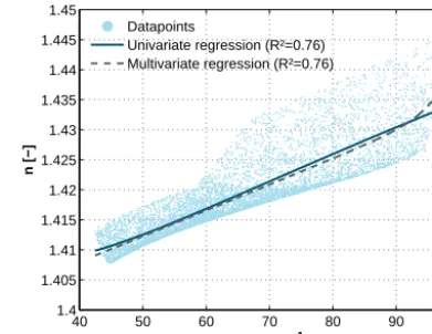
Both the shape of the obtained fits of the multivariate method and the R2 turned out to be very similar to those of the univariate method. The averageR2 both for the uni-variate and multiuni-variate method was∼0.835. The shapes of the functions differ just slightly or are even identical. Fig-ure 7 shows the univariate and multivariate regression results fornbased on the texture class Su. It can be seen that both

0 50 100 150 200

0.5 0.55 0.6 0.65 0.7 0.75 0.8 0.85 0.9 0.95

Number of classes [−]

R

2 [−]

Average R2 Range

Figure 4.Average coefficient of determination (R2) in dependency of the number of classes used for the subdivisions based on soil hydraulic properties by means of cluster analyses. The averageR2 is calculated out of theR2 of all classes for each case. For this calculation, only classes withR2>0.5 were considered. In addition to that, the range ofR2is shown. The range was calculated out of the maximum and minimumR2of the individual classes.

40 50 60 70 80 90 100 0.02

0.03 0.04

ΘR

[−]

Datapoints Regression (R²=0.99)

40 50 60 70 80 90 100

0.38 0.4 0.42

ΘS

[−]

Datapoints Regression (R²=0.93)

40 50 60 70 80 90 100

1.4 1.42 1.44

n [−]

Datapoints Regression (R²=0.76)

40 50 60 70 80 90 100

0.02 0.03 0.04

Ks [cm d−1]

α

[−]

Datapoints Regression (R²=0.63)

Figure 6.Scatterplots of the van Genuchten parameters (2R,2S, n,α) in dependency of the saturated hydraulic conductivity (Ks) for the texture class Su (silty sand) out of database 3x(variant A).

Regression functions were fitted for all variants of VGP−Ks.R2 is the coefficient of determination.

curves behave very similarly with small differences at high

Ks values. However,R2are equal to each other and a better

fit cannot be pointed out. All other comparisons between the regression results of the two methods act similar to Fig. 7. The high accordance of both methods’ results speaks for the robustness of the less elaborate univariate method. Based on this, the results of the univariate regression analyses will be used for further applications.

3.1.3 Databases 3x, variant B: classification based on

soil hydraulic properties Results of the subdivision

Figure 2 shows subdivisions of the soil texture based on soil hydraulic properties by means of cluster analyses for a num-ber of 31 classes. Results of Twarakavi et al. (2010) showed that the subdivisions based on soil hydraulic properties are similar to the US texture-based classification, especially for coarse-textured soils (sands). These similarities were not found for fine-textured soils. The results of our subdivision based on soil hydraulic properties are unlike the texture-based classification. However, this is not directly a contra-diction to Twarakavi et al. (2010). They used the US texture triangle for comparison and we used the German classifica-tion. In addition to that, the rules and conditions for the

al-40 50 60 70 80 90 100

1.4 1.405 1.41 1.415 1.42 1.425 1.43 1.435 1.44 1.445 1.45

Ks [cm d−1]

n [−]

Datapoints

Univariate regression (R²=0.76) Multivariate regression (R²=0.76)

Figure 7.Scatterplot of the van Genuchten parameternin depen-dency of the saturated hydraulic conductivity (Ks) for the texture class Su (silty sand) out of database 3x(variant A). To compare the

univariate and multivariate regression, both functions are shown in the graph.R2is the coefficient of determination.

gorithm of the cluster analyses have a high influence on the result.

Univariate regression analyses

In variant B, we concentrate on univariate regression analy-ses only. In Fig. 4 the averageR2are shown in dependency of the number of classes used for the subdivisions. As previ-ously, regression results withR2lower than 0.5 are not con-sidered. The abscissa is limited to a maximum of 200 classes. If more classes are used, the averageR2 does not increase significantly. The average R2 ranges therefore mainly be-tween 0.7 and 0.8. If we use 31 classes, which is the same number of subdivisions as the texture-based classification of the German soil classification system, the averageR2is 0.74 and 40 % of the regression results have coefficients of determination higher than 0.5. The maximum can be found for the number of 2128 classes (R2=0.82 with 49 % of the regression results with>0.5). The results of the regression analyses based on databases 3x(variant A) yielded a totalR2 of 0.88 by using nine natural texture classes and 67 % of the regression results had anR2>0.5. In addition, the applica-tion of the univariate method is faster and less elaborative. For those reasons, we will use the results of the regression analyses based on databases 3x(variant A) for further appli-cations.

3.2 Applications on soil hydraulic functions

0 0.5 1 1.5 2 2.5 3 3.5 4 -8 -6 -4 -2 0 2 Lu

log10 (|h| [cm])

log 10 (K (h ) [ c m d -1]) Min. Ks Max. Ks

0 0.5 1 1.5 2 2.5 3 3.5 4 -8 -6 -4 -2 0 2 Su

log10 (|h| [cm])

log 10 (K (h ) [ c m d -1]) Min. Ks Max. Ks

0 1 2 3 4 5

0 0.05 0.1 0.15 0.2 0.25 0.3 0.35 0.4 0.45 0.5 S

log10 (|h| [cm])

4

[-]

Min. Ks Max. Ks

0 1 2 3 4 5

0 0.05 0.1 0.15 0.2 0.25 0.3 0.35 0.4 0.45 0.5 Lu

log10 (|h| [cm])

4

[-]

Min. Ks Max. Ks

0 1 2 3 4 5

0 0.05 0.1 0.15 0.2 0.25 0.3 0.35 0.4 0.45 0.5 Su

log10 (|h| [cm])

4

[-]

Min. Ks Max. Ks

0 0.5 1 1.5 2 2.5 3 3.5 4 -15 -10 -5 0 5 S

log10 (|h| [cm])

lo g 1 0 (K (h ) [c m d -1]) Min. Ks Max. Ks

(d) (e) (f)

(a) (b) (c)

Figure 8.Impact on thepF andK(h)curves due to the univariate regression functions out of database 3x(variant A).pF is log10of the absolute pressure headh.K(h)is the hydraulic conductivity in dependency of pressure head.2=volumetric water content. The minimum and maximum saturated hydraulic conductivities (Ks) were given by Rosetta. The van Genuchten parameters were changed in dependency ofKsby means of the regression functions.(a)pFcurves for the texture class S (sand).(b, c)The same as shown in(a), but for the texture classes Su (silty sand) and Lu (silty loam).(d)Hydraulic conductivity curves for the texture class S.(e, f)The same as shown in(d), but for the texture classes Su and Lu.

Ks values were selected ranging from the minimum to the

maximum values that were obtained out of database 3x (vari-ant A). The pF curves of the texture class S are shown in Fig. 8a. Van Genuchten’snwas computed out of the regres-sion function. ThepFcurve of the regression with the small-estKs value has a clearly smoother slope compared to the

pF curve that was obtained for the largestKs value. The

lower the Ks the more moves the shape of the pF curves

in the direction of typicalpF curves for sandy soils with a fraction of silt. The curves for lowKs values tend to have a

higher usable field capacity possibly leading to higher rates of transpiration in hydrological modelling applications. The curves for the unsaturated hydraulic conductivity K(h) of the texture class S are given in Fig. 8d. The same param-eters as for the pF curves were used. Near saturation the curves of largeKsvalues are above the curves of lowKs

val-ues. This relation changes after an intersection point at pF

of ∼2, caused by the variation of van Genuchten’s nthat is directly connected to the parameterm. From the physical point of view, the shapes of the curves can be described as reasonable. The curves with lowerKs values have a higher

fraction of small pores. These fractions of small pores are able to transport water for a wider range ofpF in contrast to the curve parameterisations with highKs values. This leads

to the intersection point that changes the dominating impact factor on the conductivity curves: forpF <2, theKsvalue,

which simply scales the curve, is the dominating factor. For

pF >2, van Genuchten’smis the dominating impact factor. However, after the intersection pointK(h)is already at very low values. Therefore, the variation ofmfor sandy soils may have a small impact compared to the impact of variations of theKsvalues.

Figure 8b shows the impact of the regression results on thepF curves of the texture class Su. Similar to Fig. 8a, the curves for lowKs values have a smoother slope. In addition

to that, the modifications of van Genuchten’sαcauses the water content to drop at higherpF values for the curves of lowKsvalues compared to the curves of highKsvalues. This

behaviour is typical for texture classes that have a slightly larger fraction of fine pores than the standard Su. The usable field capacity is more or less the same for all pF curves. The impact on hydrological model applications might nev-ertheless be immense depending on the method that reduces the potential evapotranspiration to the actual one: methods based on the actual water content of the soil within the root zone probably calculate higher rates of actual evapotranspira-tion using the parameterisaevapotranspira-tion based on lowKsvalues than

using the ones of higherKsvalues. On the other hand,

meth-ods based onpF values of the soil are expected to be less affected. The impacts on the conductivity curves for the tex-ture class Su are plotted in Fig. 8e. Here again, an intersection point can be located (at apF of∼1.8). Above this pressure head, the curves of highKsvalues drop below the curves of

texture class S, the values of K(h)at the intersection point (and close below) are still high enough to enable a water movement that is not negligible. For that reason, soil water simulations are influenced, especially during dry seasons.

The pF curves for the texture class Lu are visualised in Fig. 8c. Here, a shift on the ordinate can be observed, whereas the curves for low Ks values induce higher water

contents than the curves for highKsvalues for the same

pres-sure head. This is due to the relation that was found for Lu of2Rand2S being inversely proportional toKs. However,

the variations of ncause different slopes of the curves. The impact on the reduction of the potential evapotranspiration is comparable to the impact described for the texture class Su. The impact onK(h)is primarily driven by the variations of the Ks values, as seen in Fig. 8f. The intersection point is

approximately atpF4. At this highpF,K(h)has dropped magnitudes below the saturated value.

It can be summarised that the modifications of the VGP caused by the regression results of the databases 3x (vari-ant A) lead to plausible pF curves. Further, the impact on the conductivity functions near saturation is primarily driven by the value ofKs. As theKsvalue works as a scaling factor

for the conductivity curves, this result is no surprise and not induced by the regression functions. For medium and low saturations, however, the impact is dominated by the varia-tions of the parameterisavaria-tions of the soil hydraulic funcvaria-tions that were produced by the regression functions. Especially for the texture Su (and similar ones), the impact of the regres-sion functions will have an impact on long-term hydrologi-cal model applications. Taking the soil map of Lower Sax-ony for instance, texture classes with compositions, like Su, Sl or similar classes, occupy more than one-third of the to-tal area. For many of the texture classes, all four VGP could be fitted in dependency ofKs. However, this did not always

work as seen in Table 2. Following this, the correlation ma-trices of the VGP, generated within the regression analyses of databases 3x (variant A), were taken into account more deeply. It turned out that correlations were very low between VGP that are related to Ks and VGP that are not related to

Ks. These findings indicate the admissibility of fitting less

than four VGP in dependency ofKs.

3.3 Generating subgrid spatial variability

Spatial resolutions of hydrological models mainly depend on the resolutions of the input data of soil properties and land use, respectively. These input data are often not equally re-solved in space and time (e.g. the German ATKIS database). If the model area is subdivided into polygons by the hydro-logical model, the spatial resolution is unequally distributed and given automatically by the input layers. If the model area is subdivided into raster cells, the spatial resolution is equally distributed and depends both on input layers and on the user’s interests. For latter types of models, the spatial resolution may often induce a pseudo-accuracy, because the chosen grid

size can be much smaller than most of the subdivisions of the input layers. In any case, the real spatial resolution of a hy-drological model that has to be considered for the process description is given by the spatial resolutions of the input data. In most cases these spatial resolutions are rather coarse, causing many processes that are not directly resolved by the model.

To consider the spatial variability of soil water processes that are not directly resolved by the hydrological model, the following procedure is elaborated in order to generate param-eterisations of soil hydraulic functions:

1. Acquisition of a soil map for the model area (or similar information). In this study, a German soil map of Lower Saxony is used; see Fig. 1. If not already included in the soil map, soil information has to be transformed into texture information. This study included usage of the German soil classification system; see Sponagel (2005). 2. Obtaining texture classes out of the soil map. For ex-ample, Sl with 65 % sand, 25 % silt and 10 % clay (see Table 1).

3. Random generation of trios of numbers within a range of 0–100 with the precondition that the sum of each trio has to be 100. The numbers of each trio are assigned to be a percentage fraction of sand, silt and clay.

4. Consideration of a boundary in each direction (sand, silt, clay). This study used a±5 % boundary. For exam-ple, Sl with 65±5 % sand, 25±5 % silt and 10±5 % clay. Categorisation of the random number trios into the obtained boundaries.

5. Generation of VGP sets with the software Rosetta for the obtained texture classes (categories).

6. Regression analyses between Ks values and all other

VGP for each texture class.

The total number of needed randomly generated numbers (point 3) may differ in dependency of the texture classes that are going to be analysed. The Rosetta underlying databases have more samples of sandy soils than of clayey soils (Leij et al., 1996; Nemes et al., 2001). Furthermore, some combi-nations in the texture triangle are very seldom in nature. To ensure that these disagreements do not bias the regression re-sults, only close-range (±boundary) near-natural occurring texture classes that are obtained from soil maps should be considered for the regression analyses (here: generation of database 3x(variant A); see Sect. 2.2). The boundary was as-signed to be±5 % in order to get a representative number of VGP sets for each texture class. Other values for the bound-ary were tested, whereby much lower values (e.g.±1 %) lead to a very close range of theKs values. Much higher values

texture classes). Therefore, we recommend a value of±5 % for the boundary.

At the next step, the obtained regression functions have to be applied in a hydrological model. The following procedure is recommended:

1. Assumption of a lognormal distributions for theKs

val-ues of each texture class. The mean valval-ues are given by theKs values that were obtained with Rosetta at the

centre of each texture class. The standard deviations are given by the user.

2. Calculation of variations of the other VGP by using the regression functions and theKs distribution functions.

The number of VGP sets is up to the user. At least three sets should be used. We recommend five sets by using the 10th, 30th, 50th, 70th and 90th percentiles of theKs

distribution function. More sets are possible.

3. Run the model by parallelly using the VGP sets that were obtained at the previous point 2.

Due to the fact that standard deviations of theKs values are

in most cases unknown for meso- and macroscale hydrologi-cal model applications, this parameter should be assumed by the user. Note that this is the only tuning parameter needed for the procedure presented in this study. The standard de-viations of Ks values at field scale may vary between less

than 50 % and several hundred percent and there seem to be no clear correlations to the texture classes of the anal-ysed soils; see e.g. Ciollaro and Romano (1995), Reynolds and Zebchuk (1996), Bosch and West (1998), Mohanty and Mousli (2000), Gupta et al. (2006) or Sobieraj et al. (2002). The range of the standard deviation that should be used is in-directly given by the minimum and the maximumKsvalues

that were obtained out of database 3x(variant A). Assuming a specific standard deviation, the 10th and 90th percentiles of the resultingKsdistribution still have to be within the range

ofKs values given in database 3x (variant A). If so, the hy-drological model is ready to start the simulation. If not, the regression function should either be restricted to the range of

Ks (this is recommended) or the standard deviation should

be forced to a maximum value by the model. After fulfill-ing this condition, the hydrological model is ready to start. A possibility to effectively process the VGP sets within the hydrological model is given in point 2 of the above list. We recommend to use at least three different VGP sets per soil to describe the spatially variability. However, more sets can be used likewise. It is possible to simulate the soil water move-ment for all VGP sets parallel in one simulation run of the hydrological model. Note that vertical information about soil profiles, if available by the soil map, can be handled with the same procedure as described so far. Hence, the spatial vari-ability of soil hydraulic functions can either be described as horizontal (if just texture classes without any vertical profile information is available) or horizontal and vertical (if soil profile information is also available).

These presented developments were implemented into the hydrological modelling system PANTA RHEI (Förster et al., 2012; Förster, 2013; Kreye et al., 2010, 2012; Kreye, 2015) and were used successfully in many practical applications and projects (e.g. Hölscher et al., 2014; Wurpts et al., 2014; Kreye, 2015). PANTA RHEI has been developed by the De-partment of Hydrology, Water Management and Water pro-tection, Leichtweiss Institute for Hydraulic Engineering and Water Resources, University of Braunschweig in coopera-tion with the Institut für Wassermanagement IfW GmbH, Braunschweig (LWI-HYWAG and IFW, 2012). It is a de-terministic, semi-distributed, physically based hydrological model for single events or long-term simulations. The tempo-ral discretisation is adaptive; for many applications an hourly time step is used. The spatial discretisation is divided into three levels: HRUs (hydrologic response units), subcatch-ments and gauged catchsubcatch-ments. Watersheds are the basis for the subcatchments, which contain the HRUs. This spatial dis-cretisation makes the model very flexible to account for dif-ferences in scale of the input data, similar to the mHm model of Samaniego et al. (2010). A difference between our hydro-logical model PANTA RHEI compared to many other models is the low number of model parameters that are used for cal-ibration. We work with catchment-based model parameters, which have different effects on the subcatchment scale con-trolled by physiographic characteristics. This leads to (only) 6–8 model parameters in total to calibrate the model for an area of a many hundred square kilometres.

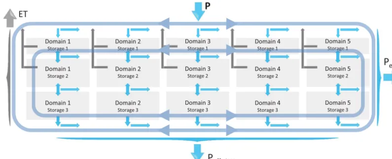
The structure of the soil model of PANTA RHEI is shown in Fig. 9. Different parameterisations of VGP (e.g. 5) are es-tablished by means of lognormal distributions ofKs. After

the sets of VGP are derived, we use all of them to param-eterise the soil model. As mentioned, we assume that one effective set of VGP cannot express subgrid variability. Sec-ondly, we assume that many different sets of VPG are able to do so. That is why the soil model is parameterised many times, whereby the structure and equations were not changed. These different models (domains) operate individually. How-ever, they are connected to each other. Summarised, it can be argued that we do not have multiple model scenarios – it is one model with multiple parameterisations solved simulta-neously. The impact of the subgrid parameterisation of the soil hydraulic functions are dominated by the variation of

Ks in wet periods and by the variation of VGP in dry

Domain1

Storage1

Domain1

Storage2

Domain1

Storage3

Domain2

Storage1

Domain2

Storage2

Domain2

Storage3

Domain3

Storage1

Domain3

Storage2

Domain3

Storage3

Domain4

Storage1

Domain4

Storage2

Domain4

Storage3

Domain5

Storage1

Domain5

Storage2

Domain5

Storage3

P

P

P

Figure 9.Application of different van Genuchten parameter sets on the soil model of the hydrological modelling system PANTA RHEI. The different parameterisations (domains) are parallel used at all spatial locations. The domains are solved simultaneously and with interaction to each other. The main input is given by the spatial precipitation (P), which was reduced in advance by vegetational interception. Results of the soil model are the direct runoff (Peff,D), the groundwater recharge (Peff,GW), which leads to base flow in a long-term view and actual evapotranspiration (ET).

data types (Gelleszun et al., 2015; Kreye, 2015). To account for the impact of the subgrid parameterisation, we compared breakthrough curves (1-D) with different numbers of VGP sets and with different standard deviations of theKs

distribu-tion funcdistribu-tions. We also compared spatially distributed sim-ulation results of the hydrological model for soil moisture with remotely sensed satellite data (ERS1/2-ESCAT, MetOp-ASCAT, ENVISAT-ASAR). The simulated soil water con-tents turned out to have high accordance with the satellite-based soil moisture. In addition to that, the model was able to approximate the dynamics of groundwater level with very high quality compared to measured data (Kreye, 2015). An-other possibility to account for subgrid variability is to anal-yse the standard deviation of soil moisture as a function of the number of applied VGP sets. Further, the spatial soil mois-ture patterns could be compared in dependence of the number of applied VGP sets, similar to Samaniego et al. (2010). We are working on a following paper focusing on the hydrologi-cal model and its hydrologi-calibration.

4 Conclusions

The objective of this study was to present a robust proce-dure to generate various sets of parameterisations of soil hy-draulic functions for the description of soil heterogeneity on a subgrid scale. To achieve this, relations betweenKsvalues

and van Genuchten’s parameters of soil hydraulic functions were investigated. The VGP were obtained with the software Rosetta. An universal function that is valid for the complete bandwidth ofKsvalues could not be found. After

concentrat-ing on natural texture classes, strong correlations were iden-tified for all parameters. The results of the numerical study presented here confirm the findings of field studies (Li et al.,

2007; Botros et al., 2009). The methodology presented in this study is applicable on a wide range of spatial scales and does not need input data from field studies.

Zhu and Mohanty (2002) tried to find effective parameters for van Genuchten’s soil hydraulic functions within a numer-ical study. They conclude that it is very difficult to define a single set of effective parameters that lead to suitable simu-lation results. In order to avoid effective parameters, the as-sumption of a parameterisation of soil hydraulic functions in dependence ofKs, as presented in this study, is a promising

alternative. Therefore, regression functions have to be set up a priori to the hydrological modelling. This is done in a much shorter time than the time needed for acquisition and prepara-tion of other input data for a large-scale hydrological model. Further, the procedure is robust in application and additional data (and costs) are not required. When using Rosetta, a soil map of the modelling area is sufficient.

It is worth discussing the applicability of transferring Rosetta results to a distributed hydrological model. An inter-change of parameters between different models can be cum-bersome. This was e.g. found by Koch et al. (2016) by using the model HYDRUS 1-D to fit VGPs, which were passed to several hydrological models (MIKE SHE, HydroGeoSphere and ParFlow-CLM). The fitting in HYDRUS 1-D was done by means of continuously measured time series of soil mois-ture at different locations and depths. HYDRUS 1-D also incorporates a Rosetta interface, but here inverse modelling was used to fit VGP. To parameterise the hydrological mod-els, Koch et al. (2016) homogeneously used the same VGP at every spatial location. In a second (heterogeneous) sce-nario they used spatially differentiated porosity (saturated water content), but all other VGP were still homogenously distributed. Hence, they nicely concluded that “future work must focus on other possibilities to further distribute the re-maining VGP parameters”. One possibility to achieve this on the mesoscale is what we introduced in our study. How-ever, we do not use another model (like HYDRUS 1-D) to estimate VGP by means of inverse modelling. Besides the need of measured input data, it is a challenge to regionalise the obtained (1-D) results of a model like HYDRUS 1-D to a spatial fully distributed hydrological model. As Rosetta is based on neural network analyses, it serves as a pedotransfer function for the estimation of VGP andKs. Data with

differ-ent levels of detail can be used as input, starting with texture classes and going up to more detailed (experimentally de-termined) information. However, Rosetta does not fit VGPs andKs by means of measured time series of e.g. soil

mois-ture or pressure head. Hence, we again want to point out that Rosetta has to be defined as “pedotransfer function” rather than using the term “model”. Compared to point measure-ments of VGP, Rosetta is not always capable to perform a perfect fit; see e.g. Pandey et al. (2005), Li et al. (2007) or Ghorbani Dashtaki et al. (2010). However, considering the huge sizes of model areas that are common for hydrologi-cal model applications, Rosetta is a good choice to generate parameters covering the complete area.

Acknowledgements. We thank the referees Yeugeniy Gusev, Anatoly Zeyliger and a anonymous referee as well as the editor Alexander Gelfan for their helpful comments and suggestions that significantly helped to improve the quality of the manuscript.

Edited by: A. Gelfan

References

Baker, F. G. and Bouma, J.: Variability of Hydraulic Conductivity in Two Subsurface Horizons of Two Silt Loam Soils, Soil Sci. Soc. Am. J., 40, 219–222, 1976.

Beven, K.: Linking parameters across scales: Subgrid parameteriza-tions and scale dependent hydrological models, Hydrol. Process., 9, 507–525, 1995.

Binley, A., Beven, K., and Elgy, J.: A physically based model of heterogeneous hillslopes: 2. Effective hydraulic conductivities, Water Resour. Res., 25, 1227–1233, 1989a.

Binley, A., Elgy, J., and Beven, K.: A physically based model of heterogeneous hillslopes: 1. Runoff production, Water Resour. Res., 25, 1219–1226, 1989b.

Blöschl, G. and Sivapalan, M.: Scale issues in hydrological mod-elling: A review, Hydrol. Process., 9, 251–290, 1995.

Boess, J., Gehrt, E., Müller, U., Ostmann, U., Sbresny, J., and Steininger, A. (Eds.): Erläuterungsheft zur digi-talen nutzungsdifferenzierten Bodenkundlichen Übersichtskarte 1 : 50.000 (BÜK50n) von Niedersachsen, Schweizerbart’sche Verlagsbuchhandlung, Stuttgart, 2004.

Bosch, D. D. and West, L. T.: Hydraulic Conductivity Variability for Two Sandy Soils, Soil Sci. Soc. Am. J., 62, 90–98, 1998. Botros, F. E., Harter, T., Onsoy, Y. S., Tuli, A., and Hopmans, J. W.:

Spatial Variability of Hydraulic Properties and Sediment Char-acteristics in a Deep Alluvial Unsaturated Zone, Vadose Zone J., 8, 276–289, 2009.

Bronstert, A. and Bárdossy, A.: The role of spatial variability of soil moisture for modelling surface runoff generation at the small catchment scale, Hydrol. Earth Syst. Sci., 3, 505–516, doi:10.5194/hess-3-505-1999, 1999.

Carsel, R. F. and Parrish, R. S.: Developing joint probability dis-tributions of soil water retention characteristics, Water Resour. Res., 24, 755–769, 1988.

Ciollaro, G. and Romano, N.: Spatial variability of the hydraulic properties of a volcanic soil, Geoderma, 65, 263–282, 1995. Coles, N. A., Sivapalan, M., Larsen, J. E., Linnet, P. E. E. R., and

Fahrner, C. K.: Modelling runoff generation on small agricul-tural catchments: can real world runoff responses be captured?, Hydrol. Process., 11, 111–136, 1997.

de Roo, A. P. J., Offermans, R. J. E., and Cremers, N. H. D. T.: Lisem: A single-event, physically based hydrological and soil erosion model for drainage basins. II: Sensitivity analysis, val-idation and application, Hydrol. Process., 10, 1119–1126, 1996. de Rooij, G. H. D., Kasteel, R. T. A., Papritz, A., and Fluhler, H.: Joint Distributions of the Unsaturated Soil Hydraulic Parameters and their Effect on Other Variates, Vadose Zone J., 3, 947–955, 2004.

Durner, W. and Flühler, H.: Soil Hydraulic Properties, in: Encyclo-pedia of Hydrological Sciences, edited by: Anderson, M. G. and McDonnell, J. J., John Wiley & Sons, Ltd, Chichester, UK, 2006. Entin, J. K., Robock, A., Vinnikov, K. Y., Hollinger, S. E., Liu, S., and Namkhai, A.: Temporal and spatial scales of observed soil moisture variations in the extratropics, J. Geophys. Res., 105, 11865–11877, 2000.

Feddes, R. A., Kowalik, P., Kolinska-Malinka, K., and Zaradny, H.: Simulation of field water uptake by plants using a soil water de-pendent root extraction function, J. Hydrol., 31, 13–26, 1976. Förster, K.: Detaillierte Nachbildung von Schneeprozessen in der

Univer-sität Braunschweig, Leichtweiß-Institut für Wasserbau, Braun-schweig, 2013.

Förster, K., Gelleszun, M., and Meon, G.: A weather dependent ap-proach to estimate the annual course of vegetation parameters for water balance simulations on the meso- and macroscale, Adv. Geosci., 32, 15–21, doi:10.5194/adgeo-32-15-2012, 2012. Gelleszun, M., Kreye, P., and Meon, G.: Lexikografische

Kalib-rierungsstrategie für eine effiziente Parameterschätzung in hochaufgelösten Niederschlag-Abfluss-Modellen, Hydrologie und Wasserbewirtschaftung, 59, 84–95, 2015.

Ghorbani Dashtaki, S., Homaee, M., and Khodaverdiloo, H.: Derivation and validation of pedotransfer functions for estimat-ing soil water retention curve usestimat-ing a variety of soil data, Soil Use Manage., 26, 68–74, doi:10.1111/j.1475-2743.2009.00254.x, 2010.

Goodrich, D. C.: Geometric simplification of a distributed rainfall-runoff model over a range of basin scales, University of Arizona, Tucson, 1990.

Gupta, N., Rudra, R. P., and Parkin, G.: Analysis of spatial variabil-ity of hydraulic conductivvariabil-ity at field scale, Can. Biosyst. Eng., 48, 155–162, 2006.

Hasenauer, S., Komma, J., Parajka, J., Wagner, W., and Blöschl, G.: Bodenfeuchtedaten aus Fernerkundung für hydrologische An-wendungen, Österr. Wasser Abfallwirt., 61, 117–123, 2009. Hillel, D.: Environmental soil physics, Academic Press, San Diego,

CA, 1998.

Hölscher, J., Petry, U., Anhalt, M., Meyer, S., Meon, G., Kr-eye, P., Haberlandt, U., Fangmann, A., Berndt, C., Wallner, M., Lange, A., and Eggelsmann, F.: Globaler Klimawandel: Wasser-wirtschaftliche Folgenabschätzung für das Binnenland: Niedrig-wasser, in: vol. 36 of Oberirdische Gewässer, 1st Edn., NLWKN, Norden, 2014.

Hopmans, J. W., Nielsen, D. R., and Bristow, K. L.: How use-ful are small-scale soil hydraulic property measurements for large-scale vadose zone modeling?, in: Environmental Mechan-ics: Water, Mass and Energy Transfer in the Biosphere, vol. 129 of Geophys. Monogr. Ser., AGU, Washington, D.C., 247–258, doi:10.1029/129GM20, 2002.

Kirchner, J. W.: Getting the right answers for the right rea-sons: Linking measurements, analyses, and models to advance the science of hydrology, Water Resour. Res., 42, W03S04, doi:10.1029/2005WR004362, 2006.

Koch, J., Cornelissen, T., Fang, Z., Bogena, H., Diekkrüger, B., Kollet, S., and Stisen, S.: Inter-comparison of three distributed hydrological models with respect to seasonal variability of soil moisture patterns at a small forested catchment, J. Hydrol., 533, 234–249, 2016.

Kreye, P.: Mesoskalige Bodenwasserhaushaltsmodellierung mit Nutzung von Grundwassermessungen und satellitenbasierten Bodenfeuchtedaten, Braunschweig, 2015.

Kreye, P., Gocht, M., and Förster, K.: Entwicklung von Prozess-gleichungen der Infiltration und des oberflächennahen Abflusses für die Wasserhaushaltsmodellierung, Hydrol. Wasserbewirt., 54, 268–278, 2010.

Kreye, P., Gelleszun, M., and Meon, G.: Ein landnutzungssen-sitives Bodenmodell für die meso- und makroskalige Wasser-haushaltsmodellierung, in: Wasser ohne Grenzen, vol. 31, edited by: Weiler, M., Forum für Hydrologie und

Wasserbe-wirtschaftung Heft 31.12, Rombach Druck- und Verlagshaus GmbH & Co. KG, Freiburg/Breisgau, 2012.

Kutílek, M. and Nielsen, D. R.: Soil hydrology, Catena-Verlag, Cremlingen-Destedt, 1994.

Lauren, J. G., Wagnet, R. J., Bouma, J., and Wosten, J. H. M.: Variability of Saturated Hydraulic Conductivity in A Glossaquic Hapludalf With Macropores, Soil Science, 145, 20–28, 1988. Law, J.: A Statistical Approach to the Interstitial Heterogeneity of

Sand Reservoirs, T. AIME, 1944, 202–222, 1944.

Leij, F., William, J., van Genuchten, M., and Williams, J.: The UNSODA unsaturated soil hydraulic database: user’s manual, EPA 600/R, National Risk Management Research Laboratory, Office of Research and Development, US Environmental Protec-tion Agency, Cincinnati, Ohio, 1996.

Li, Y., Chen, D., White, R. E., Zhu, A., and Zhang, J.: Estimating soil hydraulic properties of Fengqiu County soils in the North China Plain using pedo-transfer functions, Geoderma, 138, 261– 271, 2007.

LWI-HYWAG and IFW: Panta Rhei Benutzerhandbuch – Program-mdokumentation zur hydrologischen Modellsoftware, unveröf-fentlicht, Braunschweig, 2012.

Mallants, D., Mohanty, B. P., Vervoort, A., and Feyen, J.: Spatial analysis of saturated hydraulic conductivity in a soil with macro-pores, Soil Technol., 10, 115–131, 1997.

Marquardt, D.: An algorithm for least-squares estimation of nonlin-ear parameters, J. Soc. Indust. Appl. Math., 11, 431–441, 1963. Mohanty, B. P. and Mousli, Z.: Saturated hydraulic conductivity and

soil water retention properties across a soil-slope transition, Wa-ter Resour. Res., 36, 3311–3324, 2000.

Mualem, Y.: A new model for predicting the hydraulic conductivity of unsaturated porous media, Water Resour. Res., 12, 513–522, 1976.

Nemes, A., Schaap, M., Leij, F., and Wösten, J.: Description of the unsaturated soil hydraulic database UNSODA version 2.0, J. Hy-drol., 251, 151–162, 2001.

Pandey, N. G., Chakravorty, B., Kumar, S., and Mani, P.: Compar-ison of estimated saturated hydraulic conductivity for alluvial soils, J. Indian Assoc. Hydrolog., 28, 59–72, 2005.

Peters, A. and Durner, W.: Improved estimation of soil water reten-tion characteristics from hydrostatic column experiments, Water Resour. Res., 42, W11401, doi:10.1029/2006WR004952, 2006. Rawls, W. J., Ahuja, L., Brakensiek, D., and Shirmohammadi, A.:

Infiltration and soil water movement, in: Handbook of hydrology, edited by: Maidment, D. R., McGraw-Hill, New York, NY, 1993. Reynolds, W. D. and Zebchuk, W. D.: Hydraulic Conductiv-ity in a Clay Soil: Two Measurement Techniques and Spa-tial Characterization, Soil Sci. Soc. Am. J., 60, 1679–1685, doi:10.2136/sssaj1996.03615995006000060011x, 1996. Rossi, C. and Nimmo, J. R.: Modeling of soil water retention from

saturation to oven dryness, Water Resour. Res., 30, 701–708, 1994.

Sachs, L.: Angewandte Statistik: Anwendung statistischer Metho-den; mit 317 Tabellen und 99 Übersichten, 11. überarb. und ak-tualisierte aufl edn., Springer, Berlin, 2004.

Samaniego, L., Kumar, R., and Attinger, S.: Multiscale pa-rameter regionalization of a grid-based hydrologic model

at the mesoscale, Water Resour. Res., 46, W05523,

Schaap, M. G. and Bouten, W.: Modeling water retention curves of sandy soils using neural networks, Water Resour. Res., 32, 3033– 3040, 1996.

Schaap, M. G., Leij, F. J., and van Genuchten, M. T.: Neural Network Analysis for Hierarchical Prediction of Soil Hydraulic Properties, Soil Sci. Soc. Am. J., 62, 847–855, 1998.

Schaap, M. G., van Leij, J. F., and van Genuchten, M. T.: ROSETTA: a computer program for estimating soil hydraulic parameters with hierarchical pedotransfer functions, J. Hydrol., 2001, 163–176, 2001.

Sharma, M. L., Gander, G. A., and Hunt, C. G.: Spatial variability of infiltration in a watershed, J. Hydrol., 45, 101–122, 1980. Sobieraj, J. A., Elsenbeer, H., Coelho, R. M., and Newton, B.:

Spa-tial variability of soil hydraulic conductivity along a tropical rain-forest catena, Geoderma, 108, 79–90, 2002.

Sponagel, H.: Bodenkundliche Kartieranleitung: Mit 103 Tabellen, 5. verbesserte und erweiterte auflage edn., Schweizerbart, Stuttgart, 2005.

Twarakavi, N. K. C., Šim˚unek, J., and Schaap, M. G.: Can textubased classification optimally classify soils with re-spect to soil hydraulics?, Water Resour. Res., 46, W01501, doi:10.1029/2009WR007939, 2010.

van Genuchten, M. T.: A Closed-form Equation for Predicting the Hydraulic Conductivity of Unsaturated Soils, Soil Sci. Soc. Am. J., 44, 892–898, 1980.

van Genuchten, M. T. and Nielsen, D. R.: On Describing And Pre-dicting The Hydraulic Properties Of Unsaturated Soils, Annales Geophysicae, 615–628, 1985.

Vauclin, M., Elrick, D. E., Thony, J. L., Vachaud, G., Revol, P., and Ruelle, P.: Hydraulic conductivity measurements of the spatial variability of a loamy soil, Soil Technol., 7, 181–195, 1994.

Viera, S. R., Ngailo, J. A., Falci Dechen, S. C., and Siqueira, G. M.: Characterizing the Spatial Variability of Soil Hydraulic Proper-ties of a Poorly Drained Soil, World Appl. Sci. J., 12, 732–741, 2011.

Wösten, J. H. M. and van Genuchten, M. T.: Using Texture and Other Soil Properties to Predict the Unsaturated Soil Hydraulic Functions, Soil Science Society of America Journal, 52, 1762, 1988.

Wösten, J. H. M., Bouma, J., and Stoffelsen, G. H.: Use of Soil Survey Data for Regional Soil Water Simulation Models, Soil Sci. Soc. Am. J., 49, 1238–1244, 1985.

Wösten, J. H. M., Bannink, M. H., Gruijter, J. J. d., and Bouma, J.: A procedure to identify different groups of hydraulic-conductivity and moisture-retention curves for soil horizons, J. Hydrol., 86, 133–145, 1986.

Wurpts, A., Berkenbrink, C., Bruss, G., Dissayanake, P., Grabe-mann, I., Grashorn, S., Groll, N., Herold, M., Kaiser, R., Knaack, H., Kreye, P., Kuhn, K., Kuhn, M., Lettmann, K., Lüdecke, G., Mayerle, R., Meon, G., Miani, M., Ptak, T., Riedel, G., Ritzmann, A., Schlurmann, T., Schmidt, A., Striegnitz, M., von Storch, H., Weisse, R., Willert, M., Wolff, J.-O., Zorndt, A., and Niemeyer, H.: Forschungs-thema 7: Küste und Küstenschutz – A – Küst, in: Abschluss-bericht des Forschungsverbundes KLIFF – August 2014, edited by: Beese, F. and Aspelmeier, S., Göttingen, http: //www.kliff-niedersachsen.de.vweb5-test.gwdg.de/wp-content/ uploads/2009/05/Abschlussbericht-KLIFF-mit-Einband1.pdf (last access: June 2016), 2014.