www.hydrol-earth-syst-sci.net/18/981/2014/ doi:10.5194/hess-18-981-2014
© Author(s) 2014. CC Attribution 3.0 License.
Hydrology and
Earth System
Sciences
A spatial bootstrap technique for parameter estimation of rainfall
annual maxima distribution
F. Uboldi*, A. N. Sulis1, C. Lussana2, M. Cislaghi1, and M. Russo1
1ARPA Lombardia, Regional Hydrographic Service, Milano, Italy
2Norwegian Meteorological Institute, Climatology Division, Oslo, Norway *Independent researcher, Milano, Italy
Correspondence to: F. Uboldi ([email protected])
Received: 31 July 2013 – Published in Hydrol. Earth Syst. Sci. Discuss.: 23 September 2013 Revised: – Accepted: 2 February 2014 – Published: 11 March 2014
Abstract. Estimation of extreme event distributions and depth-duration-frequency (DDF) curves is achieved at any target site by repeated sampling among all available rain-gauge data in the surrounding area. The estimate is com-puted over a gridded domain in Northern Italy, using pre-cipitation time series from 1929 to 2011, including data from historical analog stations and from the present-day automatic observational network. The presented local regionalisation naturally overcomes traditional station-point methods, with their demand of long historical series and their sensitivity to very rare events occurring at very few stations, possi-bly causing unrealistic spatial gradients in DDF relations. At the same time, the presented approach allows for spa-tial dependence, necessary in a geographical domain such as Lombardy, complex for both its topography and its climatol-ogy. The bootstrap technique enables evaluating uncertainty maps for all estimated parameters and for rainfall depths at assigned return periods.
1 Introduction
Depth-Duration-Frequency (DDF) curves, as well as Intensity-Duration-Frequency (IDF) curves, are widely used to characterise frequency of rainfall annual maxima in a geo-graphical area. Such characterisation is an essential require-ment for architecture and civil engineering, from housing to large industrial plant design. Stewart et al. (1999) reviewed actual applications of estimates of rainfall frequency and estimation methods.
Recently, Svensson and Jones (2010) have reviewed meth-ods applied in 9 countries worldwide to characterise rainfall and flood return periods relevant for dam design. Most meth-ods are based on parameter estimation of Gumbel or GEV distribution and make use of a growth curve to relate a statis-tical rainfall index to a design rainfall/flood estimate (index-flood method). What is of interest for the present work is that many methods reviewed by Svensson and Jones (2010) make use of some form of regionalisation, either by spatially interpolating the distribution parameters after estimation at station points, or by using together data from homogeneous areas, either defined by geographical boundaries, or centred around a location of interest.
The idea of using an observational network to characterise a region has been exploited by Overeem et al. (2008), who use 12 stations for estimating (by L-moments and assuming stationarity) a single GEV distribution in the Netherlands, after verifying that the spatial dependence of the maximum rainfall is weak. Overeem et al. (2008) also evaluate uncer-tainties due to sample variability associated to estimation of GEV and DDF curves parameters, by making use of a bootstrap algorithm (GREHYS, 1996) to estimate standard deviations (SDV).
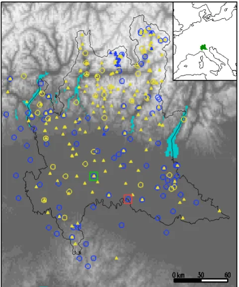
Fig. 1. Observing stations providing rainfall annual maxima in
Lombardy’s orography. Lakes are shaded in cyan. The black line shows the administrative boundary. Circles: “mechanical” stations; triangle: “automatic” stations. Yellow: less than 10 observations; blue: more than 10 observations. The inset shows the geographical position of Lombardy. The squares mark the stations discussed in Sect. 3: LODI, green, and CREMONA, red.
Regionalisation is possible when the local spatial depen-dence is weak enough to enable transferring information to a site of interest from surrounding observing sites (Buis-hand, 1991). Spatial dependence may be important, though, at a larger scale, comparable with the domain size. Lom-bardy (Italy) has a central position in the Southern Alps, it includes part of the Po Plain and, in the South, it reaches the Appennines (Fig. 1). Despite its limited spatial extension (see the distance scale in Fig. 1), Lombardy contains several different climatic areas, presenting significant rainfall differ-ences within short distances. For example, the northwestern area of Lake Como is adjacent to the area Piedmont-Ticino-Lake Maggiore, which is identified as a mesoscale hotspot for heavy precipitation in the Alps (Isotta et al., 2013). Con-versely, the eastern part of Lombardy’s Po Plain presents rather low values of mean annual precipitation (Brunetti et al., 2009).
As an example of station-point estimation in an area close to Lombardy, Borga et al. (2005) estimate DDF curves in Trentino (Italy), an area adjacent to northeastern Lombardy, assuming stationarity and making use of a simple scaling law.
After separating the dataset in convective and non-convective events, they estimate all parameters at station locations, and subsequently spatially interpolate them over the area. Sep-arately estimating at station points, however, requires the availability of long, continuous time series of reliable ob-servations at fixed sites. This can constitute a strong limi-tation in the practice, imposing a drastic reduction on the number of usable observations. In addition, as it is shown in Sect. 3 of the present document, such a station-point ap-proach is sensitive to the possible presence of rare events, which, if untreated, may cause unrealistic spatial patterns in the interpolated fields.
For these reasons, and because of the mentioned charac-teristics of Lombardy’s topography and precipitation clima-tology, it is necessary to both introduce a regionalisation and to allow for spatial dependence.
In order to estimate distribution parameters at any location, it appears appropriate to take into account all data observed at surrounding stations, at least until a prescribed distance (e.g. Reed et al., 1999), or, as in the approach presented here, with decreasing importance when distance increases. In fact, whenever time series from station sites are used to estimate DDF curves in all the points of a given area, it is implicitly assumed that each time series is representative for an area surrounding the observing station. Conversely, for any given site where an observing station is not present, all data from surrounding stations are relevant: more those from stations located nearby, less those from stations located far away. This assumption does not depend on the actual presence or ab-sence, in the present or in the past, of an observing station at the considered site.
Considering time series observed at several different sta-tions may effectively reduce the influence of outliers on pa-rameter estimation, while appropriately allowing them to in-fluence the evaluation of the estimate uncertainty. Outliers, for the underlying extreme event distribution, are events with a return period much longer than the actual length of the time series, such as very high annual maxima, representing mete-orological events that are extremely infrequent, but neverthe-less possible. Such maxima, observed very few times at very few locations may have excessive influence on distribution parameters estimated separately at each station point.
In the present work, standard estimation methods, such as L-moments and maximum likelihood, are applied to syn-thetic series generated at any desired location by resampling from several stations, irregularly distributed in space. By taking into account the length of each time series to avoid the possibility of over-sampling, the use of short time series is enabled, greatly increasing the dataset size. The method is applied over a 1.5 km×1.5 km regular grid covering the whole area of Lombardy.
Sect. 4 and results are presented in Sect. 5. Section 6 de-scribes the evaluation of uncertainty on the estimated param-eters, and discusses how this is transferred into uncertainty on the computed rainfall depth thresholds.
2 Rainfall annual maxima dataset
Data used in this study are rainfall annual maxima recorded by tipping-bucket catching gauges (Vuerich et al., 2009). Two are the main data sources: an “historical” dataset and the present-day automatic network.
The historical dataset is composed of rainfall annual max-ima from “mechanical” stations (hereafter indicated as sta-tions of type M), equipped with analog instrumentation and originally managed by the National Italian Hydrographic Service (Servizio Idrografico e Mareografico Italiano, 1917– 1998): these data were digitised in the (recent) past and are now included in the database of the Hydrographic Service at ARPA Lombardia. Data from 1929 to 2001 from 69 ob-serving sites of the historical dataset, selected with a mini-mum series length of 24 yr (in total 2753 annual records, each with 5 maxima for different event durations), were used in a study (De Michele et al., 2005) which originated the previ-ous operational scheme. In that work, a separate estimation is computed at each of the 69 stations, then a kriging spa-tial interpolation is performed to assign DDF curve parame-ters and quantiles to every location in the domain. Few more series from type M stations, not used by De Michele et al. (2005), have been recently acquired and entered the dataset. Stations of type M were manned and underwent frequent maintenance. They continued to be operational until 2005.
Since the 1990s, automatic meteorological stations (here-after indicated as stations of type A) started to be indepen-dently installed by several different public institutions, with different aims and criteria, and with inhomogeneous instru-mentation. Unfortunately, the continuity of long data series has not been guaranteed by such an important change of the observational network: the dismissal of a particular “mechan-ical” station did not automatically imply that a new auto-matic station was installed at the same location. Starting from 2004, the different existing networks merged in a single ob-servational network, the ARPA Lombardia mesonet. An op-erational quality assurance system started to be set up since 2008 (Ranci and Lussana, 2009; Lussana et al., 2010). Nowa-days, precipitation data undergo both automatic plausibility checks and human operator controls, aimed at assessing its quality and at preventing observations affected by gross er-rors from entering automatic elaborations.
The high spatial resolution of the present-day station dis-tribution is considered sufficient to appropriately describe stratiform precipitation mesoscale events, and convective events too, though with approximation depending on local station density (Lussana et al., 2009). However, the data dis-tribution is not completely homogeneous in space: border
ef-fects are likely to occur where observational information is lacking outside Lombardy; in mountain areas (Alps, Prealps and Apennines), stations are mostly located in the populated valley floors. In such areas, the estimated parameters are ex-pected to have larger uncertainty: it is then important to eval-uate it and to assess its spatial distribution, as it can be done by means of the method proposed in this document.
All data used in this study underwent supplementary quality control, including comparison of individual series with data of the same time period from other stations in the same area. Moreover, every annual maximum obtained from less than 90 % of acceptable observations in the year was rejected. Homogenisation and comparison of differ-ent data sources is still under way at ARPA Lombardia, also with the purpose of evaluating the stationarity of the statistics. In order to do that, regional averaging is recom-mended (Klein Tank et al., 2009), then the method proposed in this work might also be useful in that context. For the present study, however, stationarity has been assumed as a working hypothesis.
After quality control, with the consequent exclusion of suspect observations and even of few whole series, it has been possible to merge the historical dataset and the present-day mesoscale network. The resulting dataset ranges from 1929 to 2011. It includes 4510 annual records (each with 5 maxima for different event durations: 22 431 values, exclud-ing missexclud-ing or invalidated data) from 312 stations, shown in Fig. 1, where different symbols are used to indicate sta-tions of type M (circles, 125 stasta-tions) and A (triangles, 187 stations). The longest time series belong, of course, to sta-tions of type M. In Fig. 1, different colours are used to dis-tinguish short series, yellow (less than 10 annual maxima), from longer series, blue. The presence of short series (of both types M and A) is important both for the size of this por-tion of the dataset, and because one of the advantages of the approach presented in this work is that it enables their use, as opposed to separate station-point estimation that needs to discard them (Sect. 4).
The dataset used in this work includes annual rainfall maxima for event durationsD=1, 3, 6, 12 and 24 h.
3 Sensitivity to rare events
Figure 2 shows the time series of annual maxima for the event duration D=24 h for two stations located in the Po Plain and distant about 40 km from each other. Their loca-tions are shown in Fig. 1 as the green square, LODI, and the red square, CREMONA. The distance between these two sta-tions is rather small if compared with the expected scale of spatial variations of precipitation climatology in the Po Plain (Isotta et al., 2013; Brunetti et al., 2009).
Fig. 2. Time series of rainfall annual maxima for event duration
D=24 h for the stations: CREMONA (solid line) and LODI (dot-ted line)
observed at CREMONA correspond to infrequent, though possible, summer thunderstorms occurring in the Po Plain: the two spikes are, in fact, outliers for the annual maxima distribution.
When estimation is computed separately at each station, as in the previous operational scheme (De Michele et al., 2005) of the Hydrographic Service of ARPA Lombardia, the pres-ence of the two spikes results in important differpres-ences in the L-moments-estimated parameters of both the GEV and Gum-bel distributions and, consequently, on the quantiles. The re-sulting DDF curves are compared for the two stations in Fig. 3, where large differences can be seen, both in return periods for an assigned threshold depth, and in depths asso-ciated to an assigned probability of occurrence. It should be remarked that removing the two spikes from both series re-sulted in much similar extreme event distributions and DDF curves. Finally, the estimation has been repeated using the maximum likelihood method and the resulting DDF curves (not shown) still show a similar sensitivity to the presence of the two spikes in CREMONA’s series.
Another difference between the two series, appearing from Fig. 2, is that observations start about 30 yr earlier at CREMONA. However, discarding the first part of CRE-MONA’s series so that the two samples have comparable size (i.e. length in time), does not change the parameter estima-tion in a way comparable with the effect of the two spikes.
[image:4.595.306.548.62.232.2]The differences found in the estimated probability of rain-fall events at LODI and CREMONA are not justified for sites that are so close to each other and so similar to each other, with regard to the surrounding orography. Moreover, estimat-ing parameters of the rainfall annual maxima distributions at station locations is only an intermediate step towards charac-terising the occurrence probability of extreme rainfall events for the whole Lombardy. In other words, station data need to be used to characterise every point in the area. Any place
Fig. 3. Depth-Duration-Frequency curves for return periodsT =
100 yr (thick lines) andT =20 yr (thin lines) for the stations: CRE-MONA (solid lines) and LODI (dotted lines). The assumed distri-bution is GEV and its parameters have been estimated by the L-moments method, separately on each station.
which is close enough to both LODI and CREMONA sta-tion is expected, as a result of stasta-tion-point estimasta-tion, to be influenced by both time series in a way that rapidly vary in space, because of the occurrence of two outliers.
4 Spatial bootstrap technique
With the purpose of estimating extreme value statistical dis-tribution parameters (Sect. 4.4) in any point X (defined by its geographical coordinates), data observed at several sur-rounding stations are taken into account. At each target point X, the spatial bootstrap procedure can be sketched as follows. 1. Sampling (details in Sect. 4.1): observations from dif-ferent time series are used to resample a new, synthetic, “time series”, which is attributed to point X.
2. Parameter estimation (details in Sect. 4.2): the syn-thetic series is used to estimate scale invariance param-eters (Sect. 4.4) and distribution paramparam-eters, by means of algorithms such as L-moments (Hosking, 1990) or maximum likelihood (Coles, 2001).
3. Points (1, sampling) and (2, parameter estimation) are repeated several times (1000 in the case of the pre-sented results) to obtain, for each parameter, a distri-bution of estimates: the mean of such distridistri-bution is finally used as the actual estimate, while the standard deviation (SDV) measures its associated uncertainty, due to sample variability.
a simple scaling law (Sect. 4.4), even if they do influence the obtained estimate, are critically required for the spatial bootstrap technique, which can be applied using alternative assumptions as well.
4.1 Sampling
An ensemble of prescribed sizeMof observed values is ex-tracted randomly among all theN available data. The prob-ability of extraction of each observation is proportional to a prescribed functionγ of the distance between station loca-tion and point X. In the present case, a funcloca-tion with Gaus-sian shape is used. If thenth observation has been taken at theknth station, then:
γn=exp (
−1 2
d (X, k n) Dh 2) ·exp ( −1 2 z−z
kn Dv
2) , (1)
whered (X, kn)is the horizontal distance between stationkn and point X,z andzkn are the elevations above mean sea level, respectively of point X and of stationkn.DhandDvare
scale parameters which have been set atDh=30 km
(hori-zontal scale) andDv=600 m (vertical scale). These values,
constrained from below by the observational network resolu-tion, are chosen to impose a weak smoothing (Uboldi et al., 2008). By Eq. (1), time series from stations nearby are more frequently sampled from, with respect to time series from stations located far away from X. Remark that the chosen function accounts for elevation difference as well, and that distance-dependent probabilities are assigned to individual observations, rather than to stations, to avoid oversampling from “short” time series located near the target point X.
In traditional estimation, separately performed at each sta-tion point, “short” time series (series with few annual max-ima) are necessarily discarded, because they do not provide a sufficient number of data for the estimation. Moreover, they are useless for “long” return period, with the practical rule that the maximum significant return period is about twice the series length. Many data would be discarded in this way, in particular from stations which have been installed recently.
With the proposed method the use of very short time se-ries is enabled. For each location X (gridpoint or station), by prescribing distance-dependent extraction probabilities, observations from nearby stations are selected more often than observations from stations located far away. Oversam-pling from nearby stations with only few data is effectively avoided. In fact, if a station were chosen with probability proportional to its associatedγ and, for the selected station, an observation were chosen with uniform probability after-wards, then nearby observing locations with only few ob-servation could be over-sampled: the same few obob-servations could be chosen many times in each synthetic series. This is avoided by assigning distance-dependent probabilities to individual observations, rather than to stations, and
normal-ising with the sum of probabilities of all observed values:
0= N X n=1
γn (2)
In this way, all observations from the same station still have the same probability, but the probability of extracting from a particular station depends both on distance and on the size of its observation set, i.e. the length of its time se-ries. For example, if, for a particular location only two sta-tions existed: “a” with only 3 observasta-tions, but very close, withγa=0.9; and “b” far away, withγb=0.1, but with 100 observations, then the sum of all (observational)γs would be0=3×0.9+100×0.1=12.7. The individual probabil-ity would be 0.9/12.7 for each observation from “a” and 0.1/12.7 for each observation from “b”, but the “station” probability would be 2.7/12.7 for station “a” and 10/12.7 for station “b”.
Appendix A describes how the γs and their sum (over all observations) are used, starting from a pseudo-random real number extracted with uniform probability in the interval(0,1).
The total number of available observations is aboutN= 4500 (slightly different for each duration because of missing data, Sect. 2).
The length of the synthetic series obtained (i.e. the sample size) for the presented results (Sect. 5) isM=50, consid-ered sufficient to obtain stable estimates and to span the time period covered by the dataset (1929–2011). A larger size, M=100 has been tested, without any noticeable difference in estimates.
4.2 Parameter estimation
Parameter estimation is obtained for each synthetic series, i.e. at each gridpoint, by applying the L-moments algorithm first, then using the L-moments estimate to initialise a max-imum log-likelihood estimation, solved by means of a non-linear conjugate gradient iteration.
Since the GEV distribution (Sect. 4.4) has a lower bound whenξ >0, and a higher bound when whenξ <0, it may well happen that one or more observationw in the sample do not satisfy the condition 1+ξ (w−ε) /α >0 (Sect. 4.4) for some set of parameters(ε, α, ξ )possibly met after the L-moments estimation, or during the iterative minimisation. It has then been necessary to make sure that, before starting the line minimisation required at each conjugate gradient itera-tion step (Press et al., 1992), the sought minimum was effec-tively “bracketed” by two points, i.e. two sets of parameters (ε, α, ξ ), both satisfying the GEV condition.
4.3 Stationarity
the results presented in Sect. 5. On the contrary, if stationarity were an issue, sampling could be performed by prescribing extraction probabilities that effectively ensure uniformity in time (for example, by extracting one observation, or a fixed number of them, for each year). In that case the time coordi-nate could be used in the estimation, for example by prescrib-ing a linear dependence on time of one or more distribution parameters, in order to estimate a trend when applying the maximum-likelihood method (Coles, 2001).
4.4 Depth-Duration-Frequency curves and scale invariance
The cumulative GEV (Generalised Extreme Value) distribu-tion is:
F (h)=exp "
−
1+ξh−µ σ
−1/ξ#
, (3)
whereµ,σandξare known as the location, scale and shape parameters, respectively. The GEV expression is defined for 1+ξ (h−µ) /σ >0 and includes Gumbel distribution as the particular caseξ =0 (Wilks, 2011; Coles, 2001).
If 1−F (h)is interpreted as the probability that, in a year, a rainfall event (of a given duration) exceeds the “threshold” h, then the return period is measured in years and defined as:
T (h)≡ 1
1−F (h). (4)
The proposed spatial bootstrap method is quite general and does not depend on particular assumptions with regard to scaling. Stochastic self similarity, or multifractality, is ac-knowledged as the general scale invariance condition for rainfall fields (Veneziano et al., 2006). Here, as a working hy-pothesis for the operational implementation, we follow Bur-lando and Rosso (1996) and De Michele et al. (2005). Rain-fall annual maxima follow a scale invariance law such that the statistical distribution for an event durationλD, and that of the reference durationDare the same after scaling by a powerλn, with exponentnto be determined depending on the process and on the site. Quantiles and momenta of the dis-tribution scale then with the same factorλn. This corresponds to assuming that time series related to different event dura-tions for the same site, after normalisation with the mean, are sampled from the same extreme event statistical distribution. IfhD is the sample mean for event durationD, the distribu-tion parameters are redefined as:
ε≡ µ hD
(5)
α≡ σ hD
(6)
The same is done for the quantiles: wT ≡
hT
hD
(7) By inverting the expression of cumulative distribution func-tion, Eq. (3), the normalised rainfall depth threshold is ex-pressed as a function of the return period:
wT =ε− α ξ ( 1− ln T T −1
−ξ)
. (8)
The analytical DDF curve expression for durationD is, finally:
hT(D)=a1wTDn (9)
The scale invariance coefficient,a1, and the scaling
expo-nent,n, are obtained by least square optimisation:
n=
(lnD− hlnDi) lnhD−lnhD
(lnD− hlnDi)2 (10)
a1=exp lnhD−nhlnDi, (11)
where the averageshiare taken on event durations.
The assumption that standardized maxima of precipitation follow the GEV model with constant parameters is based on standard asymptotic results from Extreme Value theory (Coles, 2001).
Making use of a simple scaling law such as Eq. (9), though, is not mandatory.
In recent works (Veneziano et al., 2009; Langousis et al., 2013) a GEV with shape parameterξdependent on duration is advocated as the most appropriate distribution for rain-fall annual maxima and for durations of finite length. We remark that, by means of the spatial bootstrap technique pro-posed here, the sensitivity to outliers is effectively reduced (Sect. 5), the sampling size is increased (M=50, Sect. 4.1) and the final estimate for each parameter is obtained as the sample mean, effectively reducing uncertainty. The shape pa-rameterξ remains however the most uncertain (Sect. 6): al-lowing a direct dependence on duration might improve the accuracy of the estimate.
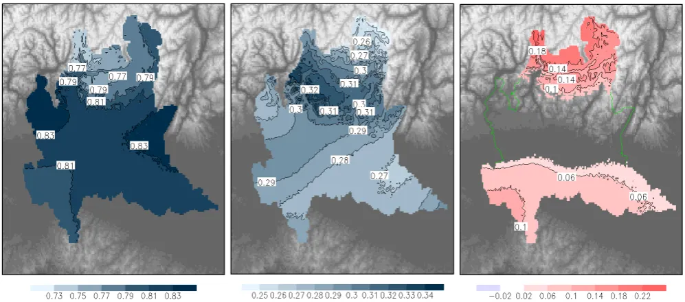
Fig. 4. Left: map of the estimated scale invariance coefficienta1(mm). Right: map of the estimated scaling exponentn(dimensionless).
[image:7.595.48.547.400.620.2]Fig. 6. Distributions of rainfall depth thresholds (mm) obtained forT =200 yr andD=3 h (left panel),D=24 h (right panel). Boxplot labelled A refers, in both panels, to the previous operational method, i.e. separate estimation at each of 69 stations; boxplot B is obtained by applying the proposed method using the same 69 stations only; boxplot C is obtained estimating at the same 69 locations, by applying the proposed method using the complete dataset. Comparing boxplot A and B shows the effect of applying the new method at the same dataset, while comparing boxplot B and C shows the effect of the dataset extension (when estimating at the same, old 69 sites). The combined effect of the method change and of the dataset extension is seen by comparing boxplot A and C.
in fact, annual maxima from convective and non-convective events are separately treated. Such criticism could lead us, in the future, to refine the scale invariance assumption, by test-ing the appropriateness of separattest-ing the 1 h duration from the rest of the dataset, or by replacing Eq. (9) with an alter-native expression, or again allowing a direct dependence on duration of the distribution parameters.
5 Estimated parameters and quantiles
The estimates of the scale invariance coefficienta1 and of
the scaling exponent n are shown as maps in Fig. 4. Fig-ure 5 shows the GEV distribution parameters: “location”ε (left panel), “scale” α(central panel) and “shape”ξ (right panel). For all these maps, the estimate is obtained as the mean of the ensemble of estimates computed by repeating 1000 times the resampling and estimation procedure at each gridpoint.
Since scale invariance has been assumed and Eqs. (5)–(7) have been used, GEV location parameterε and GEV scale parameterα(Fig. 5) are dimensionless: the only dimensional parameter is the scale invariance coefficienta1(left panel in
Fig. 4), measured in mm and representing the average rainfall depth for unity event duration.
The shape parameterξ assumes values around zero: the GEV distribution reduces to a Gumbel distribution (with the same location and scale parameters) in the limitξ=0. The estimate ofξis obtained by the mean, and the uncertainty on the estimate is evaluated by the SDV: this information is used
in the right panel of Fig. 5: the field is masked out when the absolute value of the mean is smaller than the corresponding SDV. In this way the unshaded (masked) areas are attributed to a Gumbel distribution and areas shaded in red to a “heavy-tailed” Frechét distribution. No negative values of the mean exceed, in absolute value, the corresponding SDV, then no gridpoints are attributed to a reversed Weibull distribution.
For a numeric comparison with the previous operational scheme, the presented method has been applied to the same “old” dataset, composed by 69 stations, used by De Michele et al. (2005) and described in Sect. 2. These results are shown in Fig. 6, where each boxplot shows the distribution of the rainfall depth threshold hT values estimated for the return periodT =200 yr at the 69 sites: boxplot labelled A corre-sponds to the previous operational scheme (De Michele et al., 2005), i.e. separate estimation at each station; boxplot B is obtained by using the same dataset, but with the new method described in Sect. 4; boxplot C is obtained by applying the new method to the complete dataset described in Sect. 2, but only estimating, in this case, at the 69 sites composing the old dataset. The two panels of Fig. 6 refers to event duration D=3 h, left, and to event durationD=24 h, right. The two durations are chosen as representative of annual maxima due to mainly convective events, in the case ofD=3 h, and of longer, stratiform events, in the case ofD=24 h.
Remark that possible deformations due to the interpolation step of the old method are excluded in this comparison.
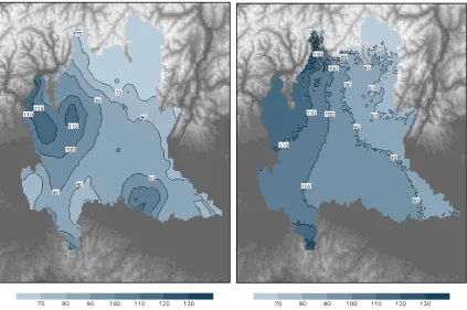
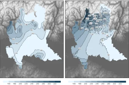
Fig. 7. Raindepth thresholdhT (mm) for event durationD=3 h and return period T=200 yr. Left panel: estimate obtained with the previous operational scheme, based on station-point estimation at 69 sites and subsequent interpolation. Right panel: estimate obtained by applying the proposed method to the same 69 stations.
dataset extension with the same, new, method. The cumula-tive effect of method change and dataset extension can then be seen by comparing boxplot A and boxplot C. The most relevant effects are, in both panels: the upward shift of the box (first to third quartiles including the median) from box-plot A to boxbox-plot B, when the estimation is influenced by nearby stations, and the progressive dispersion decrease, as measured by the decreasing interquartile range (box height), when going from boxplot A to boxplot B, then to boxplot C, with more and more data conditioning the estimation.
The root-mean-square differences between estimates at the 69 sites for the three schemes are shown in Table 1, showing that method change and dataset extension do have an impact, larger for method change.
Comparing the scheme performances at a common sub-set of observing sites has the advantage of excluding from the analysis most effects of local differences in spatial data density and of differences in elevation above mean sea level. It is however an important goal of the present work to esti-mate over the whole of an extended and complex area such as Lombardy. The three schemes A, B and C are also compared, then, as rainfall depth threshold maps, in Figs. 7–10.
Maps of the rainfall depthhT (mm) exceeded with return periodT =200 yr are shown, for event durationD=3 h, in Fig. 7 for scheme A (left) and B (right), and in Fig. 8 for the new proposed scheme with the complete dataset, C. Similar
Table 1. Root-mean-square differences (mm) of rainfall depth
thresholds estimated at the 69 sites composing the “old” dataset, with the three schemes. A: old method, old dataset; B: new method, old dataset; C: new method, new extended dataset (but only esti-mates at the 69 sites are considered for this comparison).
RMSD (mm) D=3 h D=24 h
B-A 24 48
C-B 10 21
C-A 26 55
maps are shown, for event durationD=24 h, in Fig. 9 for scheme A (left) and B (right), and in Fig. 10 for scheme C. For schemes B and C, these maps are produced by evaluating Eq. (9) at each gridpoint and estimating all parameters by their means.
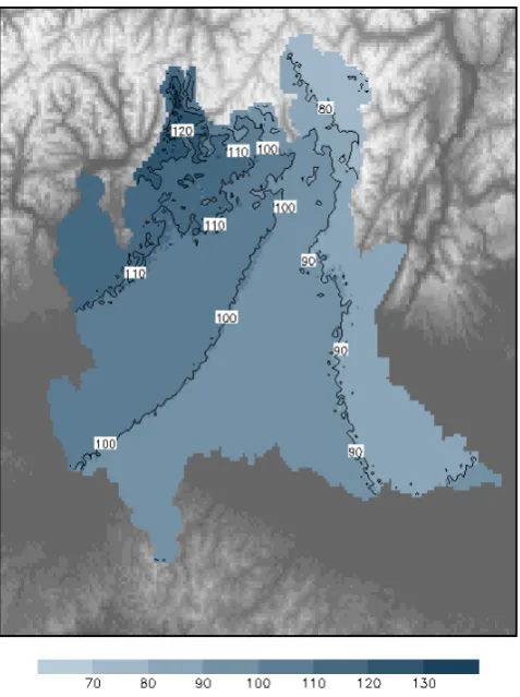
Fig. 8. Map of the rainfall depth thresholdhT (mm) for event du-rationD=3 h and return periodT =200 yr, obtained by applying the proposed method to the complete dataset.
method (both schemes B and C): rare events are effectively treated as such, by considering all surrounding data.
Since the interpolation step of scheme A does not account for elevation difference, no orographic signal can be seen in its maps. In schemes B and C, the fields appear correlated with the orographic features for durationD=24 h, associ-ated to long stratiform events, and much less for duration D=3 h, associated to important thunderstorms.
Differences between scheme B and C, due to the dataset extension, regard details of the fields. In particular, the cor-rection in the Plain discussed above is further improved by using more data in scheme C, including comparatively short time series from “recent” automatic stations, progressively installed starting from the 1990s.
It is worthwhile remarking that at the locations of the two stations discussed in Sect. 3, LODI and CREMONA (Fig. 1), the hT fields assume similar values both in Fig. 8 and in Fig. 10, and that the (weak) gradient across the Po Plain even opposes the difference found in Sect. 3 by separately estimat-ing at the two locations and, consequently, appearestimat-ing in the left panels of Figs. 7 and 9.
Table 2. Ranges of values (in the grid) of the ratio SDV/mean for a1,n,εandαand of ratio SDV/max(|mean|)forξ.
ratio SDV/mean
min max
a1(mm) 0.041 0.094 n 0.053 0.105 ε 0.015 0.048 α 0.038 0.068
ratio SDV/max(|mean|)
min max
ξ 0.172 0.325
To comment on the maps of parameters and of rainfall depth threshold estimated by applying the new proposed method to the complete extended dataset, one has to con-sider that the Alpine climatology is characterised by moist zones extending along the external flanks of the Alps and dry conditions in the interior of the mountain range (Frei and Schär, 1998). Furthermore, the western part of Lombardy’s Prealpine area is among the alpine areas with the higher val-ues of mean annual accumulated precipitation (Isotta et al., 2013; Brunetti et al., 2009). These differences are due to the complex interaction between the moist and unstable large-scale southwesterly atmospheric flows with the orography. In our study, this interaction leads to the occurrence, in the distribution parameter fields, of a south-westward gradient across the Alpine area (i.e. the northern part of the domain). This is apparent, for example, in thea1field, Fig. 4.
Conse-quently, the most exposed southwestern ridges, the Prealps, present the highesthT values in Figs. 8 and 10, while the lowesthT values are found in the shielded Alta Valtellina, the alpine area in the extreme northeast.
The Po Plain is characterised by a significant westward gradient in many parameters (for example, the a1 field in
Fig. 4), resulting in largerhT values in the west with respect to the east (Figs. 8 and 10).
Comparing hT for D=3 h, Fig. 8, and for D=24 h, Fig. 10 (both for a return period of 200 yr), the relative dif-ference between eastern and western Plain for event duration ofD=3 h appears smaller (about 20 %), than the same dif-ference relative to D=24 h (30 % at least). This could be related to the remark of Isotta et al. (2013), that in the eastern Plain a larger fraction of the mean annual accumulated pre-cipitation comes from the most intense prepre-cipitation events.
6 Uncertainty
[image:10.595.356.500.94.218.2]Fig. 9. Same as Fig. 7, but for the event durationD=24 h.
ratio between SDV and mean (i.e. the coefficient of varia-tion) of each estimated parameter, exceptξ: for this parame-ter, which has values around zero, the ratio between the SDV and the maximum of the absolute value of the mean is shown. Fora1,n,εandαthe SDV is always below or about 10 %
of the mean, so that the uncertainty on these parameter can be considered small. On the contrary, forξ, the SDV is about 40 % of the maximum (positive) value of the mean.
Uncertainty on parameters does have an impact on rainfall depth threshold. For each of the estimated parameters, the partial relative uncertainty onhT ,Dis evaluated as:
ρπ(σπ)≡
hT ,D(π+σπ)−hT ,D(π−σπ) 2hT ,D(π )
, (12)
where the generic parameterπ {a1, n, ε, α, ξ}appears and
σπ is the corresponding standard deviation. Simplified ex-pressions are easily obtained for each parameter using the scale invariance expression (Eq. 9):
ρa1=
σa1
a1
(13)
ρn=
Dσn−D−σn
2 (14)
ρπ=
wT(π+σπ)−wT(π−σπ) 2wT(π )
, (15)
[image:11.595.46.287.603.688.2]where now, in Eq. (15), π {ε, α, ξ} represents any of the three GEV parameters. As it appears in Eqs. (13)–(15), the
Table 3. Relative partial uncertainty component (%) onhT ,Dwith respect to each estimated parameter, minimum and maximum value among all gridpoints.
min MAX
a1 4.1 % 9.4 %
n(D=3 h) 2.2 % 5.0 % n(D=24 h) 6.4 % 14.4 % ε(T =20 yr) 0.72 % 1.9 % ε(T =200 yr) 0.48 % 1.1 % α(T =20 yr) 2.0 % 4.3 % α(T =200 yr) 2.6 % 5.5 % ξ(T =20 yr) 3.3 % 7.8 % ξ(T =200 yr) 7.7 % 19.3 %
a1 component of relative uncertainty onhT ,D is simply the coefficient of variation fora1; thencomponent only depends
on the duration,D; theε,αandξ components coincide with the corresponding partial components of relative uncertainty on the normalised quantilewT: they depend on the return pe-riod and on all three GEV parameter estimates, but not on the duration.
Fig. 10. Map of the rainfall depth thresholdhT (mm) for event du-rationD=24 h and return periodT =200 yr, obtained by applying the proposed method to the complete dataset.
associated to: (1) the scaling exponentnfor long event du-rations, having a maximum (over the domain) of 14.4 % for D=24 h; (2) the shape parameterξ for long return periods, reaching a maximum of 19.3 % forT =200 yr.
Figure 11 shows, as percentage, the relative uncertainty componentρξ (Eq. 15) on the rainfall depth thresholdhT ,D, for return period T =200 yr and for any duration D, due to the uncertainty on the estimate of the parameterξ. As it appears in Table 3, for long return periods this is the most important uncertainty component. It is higher in the Alpine area, where the elevation difference between gridpoints and station points effectively reduces the spatial data density with respect to its bi-dimensional appearance. Its maximum can be found in the extreme northwest (Val Chiavenna), where only few stations are located and distributed along a direc-tion which stretches outward (Switzerland) with respect to the more densely and uniformly observed part of the do-main (Fig. 1). This is a typical “border” effect, which also necessarily affects any interpolation method, and which can be easily solved by the acquisition of external observations, when they are available. Swiss observations would be neces-sary in this case, but, for Lombardy, data from other Italian departments would be very useful as well: only stations from
Fig. 11. Relative partial uncertainty componentρξ (%) on the rain-fall depth thresholdhT ,Dfor return periodT =200 yr (and for any durationD), due to the uncertainty on the estimate of the parameter ξ.
Piedmont (west) and Emilia-Romagna (south) were used in this study (Fig. 1).
Maps of uncertainty components onhT due to uncertainty on other parameters are not shown here, but all are geograph-ically distributed in a way similar toρξ (Fig. 11).
7 Conclusions
[image:12.595.308.548.66.381.2]fact, the method effectively makes use of the whole dataset, even short time series from stations recently installed, or ac-tive for only few years in the past, that must be discarded in the traditional point-by-point estimation. Uncertainties on all estimates are directly evaluated and represent an important information, both for further studies and for users.
In general, as it has been shown, parameter estimation al-gorithms are sensitive to the presence of outliers in the ob-served series. The combined use of multiple stations in the estimation enables reducing the impact of such very rare events, whereas these are appropriately allowed to affect the evaluated uncertainties.
L-moments or maximum likelihood algorithms can be in-differently applied to the synthetic series resampled at every desired location. In this work, the log-likelihood function has been maximised by means of a nonlinear conjugate gradient iteration, initialised with L-moments estimates. The whole procedure, from sampling to estimation, has been repeated 1000 times at each point of a regular 1.5 km×1.5 km grid covering the spatial domain. For each parameter, the mean and the SDV of such an ensemble of estimates provide the final estimate and its associated uncertainty, respectively.
A comparison with the previous operational scheme, based on separate station estimation, has been realised by applying the new method to the same (old) dataset and comparing the distributions of rainfall depth thresholds estimated at observ-ing sites. With the new method all quartiles values includ-ing the median are increased and includinclud-ing information from surrounding stations reduces the estimate dispersion. This is further reduced by the dataset extension enabled by spatial bootstrap.
The presence of outliers in the time series, emphasised by separate station estimation, results in unjustified gradients in rainfall depth threshold maps obtained with the old scheme. Such unrealistic signals do not appear in maps obtained with the new method presented here, as a consequence of its abil-ity to appropriately deal with outliers, in particular when the complete dataset is used.
For all event durations and return periods, the maps ob-tained by the spatial bootstrap method with the complete dataset for distribution parameters and rainfall depth thresh-olds appear in agreement with the known climatology of the geographical domain (Frei and Schär, 1998; Isotta et al., 2013; Brunetti et al., 2009), and realistically account for ele-vation above sea level.
The spatial bootstrap technique enables evaluating tainty due to sample variability. The partial relative uncer-tainty component on rainfall depth threshold with respect to each parameter has been evaluated: the largest values are found in the Alpine area, generally below 10 %, with few exceptions, notably theξ component, reaching 19 % in the extreme northwest. In principle, these results could be fur-ther improved by allowing a direct dependence on duration of the GEV shape parameter (Veneziano et al., 2009; Lan-gousis et al., 2013).
The estimated parameters and quantiles can be made avail-able to users as gridded fields, as precomputed interactive maps, for example in a web-based GIS (Geographic Infor-mation System), such as that of ARPA Lombardia (http: //idro.arpalombardia.it), or, in principle, even by allowing direct estimation at any requested location in the domain. Besides the engineering applications cited in the Introduc-tion, information on rainfall depths associated to different event durations and return periods, such as the maps shown in Figs. 8 and 10, might also be used to characterise and dif-ferentiate the critical precipitation events for Lombardy’s cli-matic areas in civil protection emergency plans. In that con-text, the availability of thresholds uncertainties is of partic-ular interest, because it enables defining precautionary alert thresholds in a realistic and statistically founded way.
Assuming stationarity and including short time series en-ables using a large amount of observations. Conversely, this relative data abundance could be used in a stationarity study, with stringent quality control and homogenisation. As a re-sult of the stationarity study, in the future both the parame-ter estimation and DDF curves might be recomputed, either assuming stationarity in a recent portion of the dataset only (the reference period 1981–2010, for example), or by allow-ing for, and estimatallow-ing, a trend in the parameters (such as GEV location and scale, for example).
Finally, as discussed in Sect. 4.4, the scale invariance for-mulation could be refined in the future to allow for a possible different behaviour of short-duration convective events and for the use of more sophisticated GEV models.
Appendix A
Random integers with assigned probabilities
Given a realisationρ of a continuous random variable uni-formly distributed on the interval(0,1), it is possible to ob-tain a discrete random variable, uniformly distributed among the positive integers up to a genericM, by means of the trans-formation:
m=1+int(ρM) , (A1)
where “int” is a function that returns the integer part of its argument, so that:
m−1≤ρM < m (A2)
Remark thatmis the smallest integer such that:
ρM−m <0 (A3)
in Sect. 4. If the probability of extraction of the positive in-tegern≤N is required to be proportional toγn(as defined by Eq. 1 in our case), than the valueρ0(where0is the sum of allγs as in Eq. 2), is associated to a uniform random vari-able defined in the interval(0, 0). The desirednsatisfies, in analogy with Eq. (A2):
n−1
X j=1
γj≤ρ0 < n X j=1
γj (A4)
Then n is the smallest integer such that (compare with Eq. A3):
ρ0− n X
j=1
γj<0 (A5)
To operationally obtain a realisationnconsistent with the de-sired random number generator, eachγj for j=1,2, . . .is sequentially subtracted fromρ0until a negative value is ob-tained whenj=n.
Acknowledgements. The constructive criticism of the two referees,
G. Pegram and A. Langousis, lead to an improvement of the article.
Edited by: L. Samaniego
References
Borga, M., Vezzani, C., and Dalla Fontana, G.: Regional rainfall depth-duration-frequency equations for an alpine region, Nat. Hazard., 36, 221–235, 2005.
Brunetti, M., Lentini, G., Maugeri, M., Nanni, T., Simolo, C., and Spinoni, J.: 1961-1990 high-resolution northern and central Italy monthly precipitation climatologies, Adv. Sci. Res., 3, 73–78, doi:10.5194/asr-3-73-2009, 2009.
Buishand, T. A.: Extreme rainfall estimation by combin-ing data from several sites, Hydrol. Sci. J., 36, 345–365, doi:10.1080/02626669109492519, 1991.
Burlando, P. and Rosso, R.: Scaling and multiscaling models of depth-duration-frequency curves for storm precipitation, J. Hy-drol., 187, 45–64, doi:10.1016/S0022-1694(96)03086-7, 1996. Coles, S.: An introduction to statistical modeling of extreme values,
Springer, 2001.
De Michele, C., Rosso, R., and Rulli, M. C.: Il regime delle precip-itazioni intense sul territorio della Lombardia, Tech. rep., ARPA Lombardia, Milano, 2005 (in Italian).
Di Baldassarre, G., Brath, A., and Montanari, A.: Reliability of different depth-duration-frequency equations for estimating short-duration design storms, Water Resour. Res., 42, W12501, doi:10.1029/2006WR004911, 2006.
Frei, C. and Schär, C.: A precipitation climatology of the Alps from high-resolution rain-gauge observations, Int. J. Climatol., 18, 873–900, 1998.
GREHYS: Inter-comparison of regional flood frequency procedures for Canadian rivers, J. Hydrol., 186, 85–103, doi:10.1016/S0022-1694(96)03043-0, 1996.
Hosking, J. R. M.: L-moments: analysis and estimation of distribu-tions using linear combinadistribu-tions of order statistics, J. Roy. Stat. Soc., 52B, 105–124, 1990.
Isotta, F. A., Frei, C., Weilguni, V., Perˇcec Tadi´c, M., Lassègues, P., Rudolf, B., Pavan, V., Cacciamani, C., Antolini, G., Ratto, S. M., Maraldo, L., Micheletti, S., Bonati, V., Lussana, C., Ronchi, C., Panettieri, E., Marigo, G., and Vertaˇcnik, G.: The climate of daily precipitation in the Alps: development and analysis of a high-resolution grid dataset from pan-Alpine rain-gauge data, Int. J. Climatol., published online, doi:10.1002/joc.3794, 2013. Klein Tank, A. M. G., Zwiers, F. W., and Zhang, X.: Guidelines
on Analysis of extremes in a changing climate in support of in-formed decisions for adaptation, WCDMP-72, WMO-TD 1500, 2009.
Langousis, A., Carsteanu, A. A., and Deidda, R.: A simple approx-imation to multifractal rainfall maxima using a generalised ex-treme value distribution model, Stoch. Environ. Res. Risk As-sess., 27, 1525–1531, doi:10.1007/s00477-013-0687-0, 2013. Lussana, C., Salvati, M. R., Pellegrini, U., and Uboldi, F.: Efficient
high-resolution 3-D interpolation of meteorological variables for operational use, Adv. Sci. Res., 3, 105–112, 2009.
Lussana, C., Uboldi, F., and Salvati, M. R.: A spatial consis-tency test for surface observations from mesoscale meteoro-logical networks, Q. J. Roy. Meteorol. Soc., 136, 1075–1088, doi:10.1002/qj.622, 2010.
Overeem, A., Buishand, A., and Holleman, I.: Rainfall depth-duration-frequency curves and their uncertainties, J. Hydrol., 348, 124–134, doi:10.1016/j.jhydrol.2007.09.044, 2008. Overeem, A., Buishand, T. A., and Holleman, I.: Extreme
rainfall analysis and estimation of depth-duration-frequency curves using weather radar, Water Resour. Res., 45, W10424, doi:10.1029/2009WR007869, 2009.
Overeem, A., Buishand, T. A., Holleman, I., and Uijlenhoet, R.: Ex-treme value modeling of areal rainfall from weather radar, Water Resour. Res., 46, W09514, doi:10.1029/2009WR008517, 2010. Press, W. H., Flannery, B. P., Teukolsky, S. A., and Vetterling, W. T.:
Numerical recipes, the art of scientific computing, Cambridge University Press, 1992.
Ranci, M. and Lussana, C.: An automated data quality con-trol procedure applied to a mesoscale meteorological net-work, in: 9th EMS Annual Meeting, 9th European Con-ference on Applications of Meteorology (ECAM) Abstracts, held 28 September–2 October, 2009 in Toulouse, France, available at: http://meetingorganizer.copernicus.org/EMS2009/ EMS2009-335.pdf (last access: 17 September 2013), 2009. Reed, D. W., Faulkner, D. S., and Stewart, E. J.: The FORGEX
method of rainfall growth estimation II: Description, Hydrol. Earth Syst. Sci., 3, 197–203, doi:10.5194/hess-3-197-1999, 1999.
Stewart, E. J., Reed, D. W., Faulkner, D. S., and Reynard, N. S.: The FORGEX method of rainfall growth estimation I: Re-view of requirement, Hydrol. Earth Syst. Sci., 3, 187–195, doi:10.5194/hess-3-187-1999, 1999.
Uboldi, F., Lussana, C., and Salvati, M.: Three-dimensional spa-tial interpolation of surface meteorological observations from high-resolution local networks, Meteorol. Appl., 15, 331–345, doi:10.1002/met.76, 2008.
Veneziano, D., Langousis, A., and Furcolo, P.: Multifractality and rainfall extremes: a review, Water Resour. Res., 42, W06D15, doi:10.1029/2005WR004716, 2006.
Veneziano, D., Langousis, A., and Lepore, C.: New asymp-totic and preasympasymp-totic results on rainfall maxima from multifractal theory, Water Resour. Res., 45, W11421, doi:10.1029/2009WR008257, 2009.
Vuerich, E., Monesi, C., Lanza, L. G., Stagi, L., and Lanzinger, E.: WMO field intercomparison of rainfall intensity gauges (Vigna di Valle, Italy, October 2007–April 2009), WMO IOM99, WMO-TD 1504, 2009.