On the uncertainties associated with using gridded rainfall data as a proxy for observed

www.hydrol-earth-syst-sci.net/16/1481/2012/ doi:10.5194/hess-16-1481-2012

© Author(s) 2012. CC Attribution 3.0 License.

Earth System

Sciences

On the uncertainties associated with using gridded rainfall data as a

proxy for observed

C. R. Tozer, A. S. Kiem, and D. C. Verdon-Kidd

Environmental and Climate Change Research Group, School of Environmental and Life Sciences, Faculty of Science and IT, University of Newcastle, NSW, Australia

Correspondence to: C. R. Tozer ([email protected])

Received: 9 September 2011 – Published in Hydrol. Earth Syst. Sci. Discuss.: 15 September 2011 Revised: 22 April 2012 – Accepted: 28 April 2012 – Published: 23 May 2012

Abstract. Gridded rainfall datasets are used in many

hy-drological and climatological studies, in Australia and else-where, including for hydroclimatic forecasting, climate attri-bution studies and climate model performance assessments. The attraction of the spatial coverage provided by gridded data is clear, particularly in Australia where the spatial and temporal resolution of the rainfall gauge network is sparse. However, the question that must be asked is whether it is suitable to use gridded data as a proxy for observed point data, given that gridded data is inherently “smoothed” and may not necessarily capture the temporal and spatial vari-ability of Australian rainfall which leads to hydroclimatic extremes (i.e. droughts, floods). This study investigates this question through a statistical analysis of three monthly grid-ded Australian rainfall datasets – the Bureau of Meteorol-ogy (BOM) dataset, the Australian Water Availability Project (AWAP) and the SILO dataset. The results of the monthly, seasonal and annual comparisons show that not only are the three gridded datasets different relative to each other, there are also marked differences between the gridded rainfall data and the rainfall observed at gauges within the corresponding grids – particularly for extremely wet or extremely dry condi-tions. Also important is that the differences observed appear to be non-systematic. To demonstrate the hydrological im-plications of using gridded data as a proxy for gauged data, a rainfall-runoff model is applied to one catchment in South Australia initially using gauged data as the source of rainfall input and then gridded rainfall data. The results indicate a markedly different runoff response associated with each of the different sources of rainfall data. It should be noted that this study does not seek to identify which gridded dataset is the “best” for Australia, as each gridded data source has its

pros and cons, as does gauged data. Rather, the intention is to quantify differences between various gridded data sources and how they compare with gauged data so that these dif-ferences can be considered and accounted for in studies that utilise these gridded datasets. Ultimately, if key decisions are going to be based on the outputs of models that use gridded data, an estimate (or at least an understanding) of the uncer-tainties relating to the assumptions made in the development of gridded data and how that gridded data compares with re-ality should be made.

1 Introduction

Rainfall data is a crucial component in many engineering applications. It is required, for example, to carry out rain-fall/runoff modelling to estimate inflows into a reservoir, de-termine the size of rainwater tanks for water sensitive ur-ban design, or calculate the size of levees for flood mit-igation strategies. Similarly, those in the climate commu-nity use rainfall data to develop and test seasonal forecast-ing schemes, perform climate attribution studies and verify climate model outputs. However, it is often the case, particu-larly in Australia due to low population densities and the rel-atively short history of observational recordings (especially away from the eastern seaboard), that observational rainfall data does not exist at the specific location of interest for such hydrological or climatological investigations. The sparseness of the rainfall observation network means that the gauge clos-est to the point of interclos-est may be several kilometres away and therefore not representative of the climate patterns at the required location (Jeffrey et al., 2001).

In order to overcome this problem, and also due to the in-creasing development and popularity of Geographical Infor-mation Systems (GIS) software and grid based climate and hydrological models, significant efforts have been made into spatially interpolating data so as to fill the “gaps” in the ob-servational network (e.g. Jeffrey et al., 2001; Hapuarachchi et al., 2008; Kiem et al., 2008; Jones et al., 2009). There are currently two Australia-wide monthly gridded rainfall datasets available. These are the Australian Water Availabil-ity Project (AWAP) dataset (http://www.eoc.csiro.au/awap/) and the SILO dataset (www.longpaddock.qld.gov.au). The AWAP dataset superseded the Bureau of Meteorology’s for-mer operational gridded rainfall dataset (referred to as the BOM dataset henceforth) in early 2010. While the BOM, AWAP and SILO gridded datasets were developed with the same objective in mind (i.e. complete spatial coverage of rainfall data for Australia), the methods used to produce the various gridded datasets differ in many aspects (refer to Sect. 2.1 for details). All three datasets have been used in recent hydrological and climatological studies. For example, the BOM gridded rainfall data was used in recent studies un-dertaken by Verdon-Kidd and Kiem (2009, 2010) and Evans et al. (2009) and the SILO dataset was used in hydrological modelling for the Murray Darling Basin Sustainable Yields and Tasmania Sustainable Yields projects (see Chiew et al., 2008; Viney et al., 2009) and is widely used in industry (e.g. environmental consulting, government agencies, water au-thorities). AWAP data was used in the modelling undertaken for the Climate Futures for Tasmania project (Grose et al., 2010) and also in several projects being undertaken as part of the South Eastern Australian Climate Initiative: Phase 2 (www.seaci.org).

As discussed, due to the spatially and temporally incom-plete nature of the observational network in Australia (and many other places in the world), continuous century (or greater) long, monthly and daily rainfall data that covers the whole of Australia is immensely attractive – as demon-strated by the widespread use of various sources of gridded data. However, it must be remembered that gridded data is in essence “virtual data” and that numerous assumptions un-derlie the spatial interpolation techniques used to produce the gridded data and that these assumptions differ across the vari-ous gridded data products. Given the “virtual” nature of grid-ded data, and the different techniques used to produce it, dif-ferences between (a) gridded data and observed gauge data and (b) the different gridded datasets will exist. The Bureau of Meteorology (2011) acknowledges that “data smoothing” occurs in the production of gridded data such that the grid-ded values will likely differ from the rainfall recorgrid-ded at the contributing gauges. Whilst Beesley et al. (2009) have re-viewed the AWAP and SILO error statistics (on a daily scale) and Jones et al. (2009) and Fawcett et al. (2010) have com-pared AWAP and BOM error statistics, comparisons of the three existing gridded datasets with individual gauges have not been made.

The aim of this study is therefore to identify where and when the differences between gridded and gauged monthly, seasonal and annual data occur and to quantify the mag-nitude of the disagreements (Sect. 4). SA is chosen as the case study as it is a region with limited gauged data and its water resources have also recently become a research focus with the establishment of the Goyder Institute (http: //www.goyderinstitute.org/index.php). Studies into SA’s wa-ter resources require rainfall data but limited work has been done on analysing the pros and cons of various sources of rainfall data for SA. Of particular interest are the poten-tial implications of using gridded rainfall data as a proxy for gauged data in hydrological modelling in SA (Sect. 5). It should be noted that this study does not seek to identify which gridded dataset is the “best” – it is unlikely this is even possible given that all data sources, including observed gauge data (e.g. Lavery et al., 1997; Jeffrey et al., 2001), have their strengths and weaknesses. Rather, the intention here is to quantify differences between various gridded data sources, and how they each compare with observed point data, such that these differences can be considered and accounted for in the increasing number of studies that utilise gridded data.

2 Data

2.1 Gridded rainfall data

The BOM, AWAP and SILO Australia-wide gridded datasets provide spatially interpolated monthly (and daily, in the case of AWAP and SILO) rainfall grids at a resolution of 0.05◦_×0.05◦_{(i.e. approximately 25 km}2_).

The original BOM gridded dataset was produced using the Barnes successive correction technique (Jones and Wey-mouth, 1997). In this technique, grid values are derived from nearby observation gauges whose influence on a grid cell is determined based on the distance between the two points. Several iterations are performed to decrease the difference between the grid cells and the observed data until a high res-olution grid is produced (Jones and Weymouth, 1997). In this case, grids at a 0.25◦longitude-latitude resolution were pro-duced (Jones and Weymouth, 1997; Fawcett et al., 2010).

longer updated, as it was superseded by the AWAP dataset in early 2010 (Fawcett et al., 2010), and therefore all analyses are restricted to this period. Again, it is important to note that the dataset referred to in this paper as the BOM dataset is not the same as the original BOM gridded rainfall dataset (Jones and Weymouth, 1997) which had a 0.25◦longitude-latitude resolution and did not employ spline interpolation.

The AWAP dataset is produced as part of the Australian Water Availability Project, a joint initiative of the BOM and the Commonwealth Scientific and Industrial Research Organisation (CSIRO). In the daily/monthly AWAP dataset the observed daily/monthly rainfall from gauges within the BOM gauging network (i.e. up to approximately 7500 gauges, both open and closed) is decomposed into a monthly average and associated anomaly (Jones et al., 2009). Anoma-lies are used as they tend to be weakly related to topogra-phy, which is important given that the current BOM gaug-ing network does not adequately resolve high elevation areas in Australia (Jones et al., 2009). The daily/monthly anoma-lies are interpolated using the Barnes successive correction technique, described above, and the monthly climatological averages are interpolated using three dimensional smooth-ing splines (Jones et al., 2009). The rainfall grids are pro-duced by multiplying the monthly climate average grids and daily/monthly anomaly grids. An unexplained microscale variance term is used in AWAP to allow for observational or measurement error, such that exact reproduction of gauged values at each gauge location is not expected (Jones et al., 2009). AWAP rainfall grids are freely available from 1900 onwards at http://www.bom.gov.au/jsp/awap/. It is noted that the AWAP product is undergoing constant improvement and development – in this study AWAP Version 3 daily interpo-lated and monthly interpointerpo-lated datasets were used (CSIRO March 2010 reformat of the Bureau of Meteorology AWAP version 3 monthly rainfall surfaces).

The SILO dataset is produced by the Queensland De-partment of Environment and Resource Management. Three SILO products are available: interpolated data grids, the data drill product (gridded data extracted at any chosen location in Australia) and the patched point data product (gauged data with missing values infilled with gridded data). In this analysis the daily and monthly data drill product and data grids, available from 1890 onwards from www.longpaddock. qld.gov.au/silo/, were used. To generate the monthly grid-ded SILO rainfall dataset, the observed data from over 5000 BOM gauges is normalised and then interpolated using ordinary kriging. The observed data is cross validated and gauges with high residuals are removed. The updated dataset is reinterpolated using ordinary kriging and the monthly rain-fall surfaces are generated by reversing the normalisation (Jeffrey et al., 2001; Jeffrey, 2006). It is important to note that the process used to create the SILO datasets is set to accu-rately reproduce the observed data (i.e. exact interpolation).

2.2 Observed rainfall data

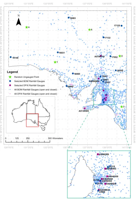
The gridded datasets described in the previous section are all based on interpolations of rainfall observed at BOM gauging gauges. The BOM rainfall gauge network in SA is compre-hensive, with close to 1600 gauges situated across the state. Many gauges offer over 100 yr of daily rainfall data and 65 of the BOM gauges are considered “high quality”, as defined by Lavery et al. (1997), who developed a list of 379 BOM rainfall gauges across Australia that did not show inhomo-geneities or spurious trends in their data records (Lavery et al., 1997; Gallant and Karoly, 2010). BOM gauged monthly rainfall totals were extracted from http://www.bom.gov.au/ climate/data/ for 16 BOM gauges across SA (see Fig. 1) that encompass a range of elevations and locations (coastal and inland) and cover various timeframes. BOM gauge details are provided in Table 1. Five of the 16 gauges are “high qual-ity” and have records greater than 70 yr. The additional 11 gauges, five “long record” (>70 yr) and six “short record” (<50 yr), although not rated as “high quality” based on the Lavery et al. (1997) definition, are on average 91 % complete and therefore suitable for this analysis.

Despite being “dependent” data (i.e. used in the develop-ment of the three gridded datasets), the BOM gauged data allows an insight into how the gridded datasets compare to gauges with long records and records for remote gauges. However, to achieve the objective of quantifying differences between various gridded data sources, and how they compare with observed point data, an “independent” reference source is needed. Hence, gauged data, not used in the development of the three gridded datasets (i.e. independent gauged data) was provided by SA’s Department for Water (DFW). The DFW manages 80 rainfall gauges in South Australia, with the majority situated in the south-eastern portion of the state (see Fig. 1). Around half of the gauges have less than 10 yr of rainfall data and many gauges have missing data. After an as-sessment of gauge locations, data record lengths and quality, 10 DFW gauges were selected for the gauged and gridded data analysis (see Sect. 3 for a description of analyses un-dertaken). The selected gauge record lengths range from 21 to 31 yr, with most gauge records commencing in the 1980s. The gauge records are on average 92 % complete. Figure 1 indicates all DFW gauges, as well as those selected for the analysis. Selected gauge details are also provided in Table 1. While the DFW gauges do not provide a complete spatial and temporal picture of rainfall in South Australia they do allow independent assessment to be made and, importantly, allow performance assessments to be made in locations not covered by BOM gauges.

2.3 Data utilised for hydrological model

Daily observed streamflow (gauge number A4260504, ob-tained from the Department for Water’s Surface Wa-ter Archive: http://e-nrims.dwlbc.sa.gov.au/swa/) and daily

Table 1. Gauged data details. Gauge numbers marked with an asterisk indicates high quality BOM gauges as given in Lavery et al. (1997).

Elevation is given in metres with respect to the Australian Height Datum (mAHD).

Gauge No. Gauge name Record Record Years Elevation Managing

start end (mAHD) agency

16031 Tarcoola (Mulgathing) Jan 1934 Open 76 198 BOM

16055∗ Yardea Nov 1877 Open 125 260 BOM

16083∗ Hamilton Gauge Feb 1931 Open 71 170 BOM

17052 Gammon Ranges (Wertaloona) Jun 1906 Open 100 100 BOM

17125 Innamincka (Bookabourdie) Jul 1997 Open 12 45 BOM

17132 Marree (Etadunna) May 1998 Open 12 30 BOM

18069∗ Elliston Feb 1882 Open 126 7 BOM

18146 Tar 639 Mile Jul 1941 Dec 1968 27 150 BOM

19001∗ Appila Feb 1882 Open 120 369 BOM

19047 Booleroo Centre (Willowie) Feb 1898 Open 109 316 BOM

20050 Plumbago Dec 1970 Open 39 260 BOM

21027 Jamestown Jan 1878 Open 123 455 BOM

23318 Tanunda Feb 1870 Open 120 250 BOM

23721∗ Happy Valley Reservoir Mar 1864 Open 119 170 BOM

23736 Mount Lofty Summit Apr 1905 Aug 1956 50 727 BOM

23808 Yundi Feb 1969 Feb 2003 34 262 BOM

A4260638 Mt Barker Creek Catchment Pluvio Jul 1984 Open 27 310 DFW A4260639 Finniss River Catchment Pluvio Aug 1985 Open 26 285 DFW

A5040552 First Creek Catchment Mar 1986 Open 25 686 DFW

A5040558 Torrens River Catchment Pluvio May 1981 Open 30 370 DFW A5040559 Sixth Creek Catchment Pluvio Jul 1983 Open 28 570 DFW A5050502 North Para River at Yaldara Nov 1985 Open 26 145 DFW A5060500 Wakefield River near Rhynie Sep 1985 Open 26 202 DFW A5080504 Baroota Reservoir Catchment Pluvio Feb 1979 Open 31 523 DFW A5100516 Aroona Dam Pluviometer Feb 1986 Open 25 236 DFW A5130505 Rocky River Catchment Pluvio Mar 1990 Open 21 133 DFW A4260504 (FLOW) Finniss River Flow Gauge Apr 1969 Open 43 203 DFW

rainfall (BOM gauge number 23808 obtained from http: //www.bom.gov.au/climate/data/) within the Finniss River catchment in SA (see Fig. 2) and mean monthly areal poten-tial evapotranspiration (from maps provided at http://www. bom.gov.au/climate/averages/climatology/evapotrans/) were used to calibrate the hydrological model (see Sect. 5 for details).

3 Methodology

3.1 Intercomparison of gridded rainfall datasets

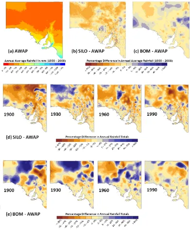
Given that the three gridded datasets (BOM, AWAP, and SILO) are produced using different methods, some differ-ences between them are to be expected. However, the gridded datasets are all intended to represent the same situation (i.e. reality) and therefore it is hoped that these differences are minimal. As a first step in understanding how the three grid-ded datasets compare, the percentage differences in annual averages for the 1900–2008 period between SILO and AWAP gridded datasets and BOM and AWAP gridded datasets for the whole of SA as well as the differences in annual totals

for the years 1900, 1930, 1960 and 1990 were determined. The comparison of annual averages was also undertaken at five randomly selected ungauged point locations within SA (see Fig. 1 for point locations). Note that AWAP was used as the reference point here as this dataset is widely used by Government agencies and the general public due to its free availability on the BOM website.

3.2 Comparison of gridded rainfall datasets against

gauged rainfall

! ! !!! ! ! !! ! ! ! !! ! !! ! ! ! ! ! ! ! !!! !!!! ! ! ! !!!! ! ! ! ! ! ! !! ! ! ! !! ! ! ! ! ! ! !! ! ! ! !! !! ! ! ! ! ! ! ! ! !! ! ! ! ! ! ! ! ! ! ! ! ! ! ! ! ! ! ! ! ! ! ! ! ! ! ! ! ! ! ! ! ! ! ! ! ! ! ! ! ! !! ! ! ! ! !! ! ! !! ! ! ! ! ! !! ! ! ! ! !! !! ! ! ! !! ! ! ! ! ! ! ! ! ! ! ! ! ! ! ! !! ! ! ! ! ! ! ! ! ! ! ! ! ! ! ! ! ! !! ! ! ! ! ! ! ! ! ! ! ! ! ! !!! ! ! ! ! ! ! ! ! ! ! ! ! ! ! ! ! ! ! ! !!!! ! ! ! ! ! !! !! ! ! ! ! !! ! !! ! ! ! ! ! ! ! ! ! ! ! ! ! ! ! ! ! ! ! ! ! ! ! ! ! ! ! ! ! ! ! ! ! ! ! ! ! ! ! ! ! ! ! ! ! ! ! !! ! ! !! ! ! ! ! ! ! ! ! ! ! ! ! ! ! ! ! ! ! ! ! ! ! ! ! ! ! ! ! ! ! ! ! !!! ! ! ! ! ! ! ! ! ! ! !! ! ! ! ! ! ! ! ! ! ! ! ! ! ! ! ! ! ! ! ! ! ! ! !! ! !! !! ! ! ! ! ! ! !! ! ! ! ! ! ! ! ! ! ! ! ! ! ! ! !! ! ! ! ! ! ! ! ! ! ! ! ! ! ! !! !! ! ! ! ! !! ! ! ! !!! ! ! !! ! !! ! ! ! ! ! !! ! ! ! ! ! ! ! !! ! ! ! ! ! ! ! ! ! ! ! ! ! ! ! ! !! ! ! ! ! ! !!!! ! ! ! !!! ! ! ! ! ! ! ! ! ! ! ! ! ! ! ! ! !! !!!! ! ! ! ! ! ! ! ! ! ! ! ! ! ! ! ! ! ! ! ! ! ! ! ! ! ! ! ! !!! ! ! ! !! !! ! ! ! ! ! ! ! ! !! ! ! ! ! ! ! ! ! ! ! ! ! ! ! ! ! ! ! ! ! ! ! ! ! ! ! ! ! ! ! ! ! ! ! ! ! ! ! ! ! ! ! ! !! ! ! ! ! ! ! ! ! ! !! ! ! ! ! ! ! !! ! !! ! ! ! ! ! !! !!! ! ! ! ! ! ! ! ! ! !! ! ! ! ! ! ! ! ! ! !! ! ! ! ! ! ! ! ! ! ! ! ! !!! ! ! ! ! ! ! ! ! ! ! ! ! ! ! ! ! ! ! ! ! ! !! ! ! ! ! ! ! ! ! ! ! ! ! ! ! ! ! ! ! ! ! ! ! ! !! ! ! ! ! ! ! ! ! ! ! ! ! !! ! ! ! ! ! ! !!! ! ! ! !! ! !!! ! ! ! ! ! ! ! ! ! ! ! ! ! ! ! !! ! ! !! ! !! ! ! ! ! ! ! ! ! ! ! ! ! ! ! ! !!! ! ! ! ! ! ! ! ! ! ! ! ! ! ! ! ! ! ! ! !!! ! ! ! !! !! ! ! ! ! ! ! ! ! ! ! ! !! ! ! ! ! ! ! !!! ! ! ! !!!! ! ! !! ! ! ! ! ! ! ! ! !!! ! ! ! ! ! ! ! ! ! ! ! ! ! ! ! ! ! ! !! ! ! !!! ! ! ! !! !! ! !! !! ! ! ! !! !! ! ! ! ! ! ! ! ! ! ! ! ! ! ! ! ! ! ! ! ! ! ! ! ! ! ! ! ! ! ! ! ! ! ! ! ! ! ! ! ! ! ! ! ! ! ! ! ! !! ! !!! ! !! ! ! ! ! ! ! ! ! ! ! ! ! ! ! ! ! ! ! ! ! ! ! ! !! !! ! !! ! ! ! ! ! ! ! ! ! ! ! ! ! !! ! ! ! ! ! ! ! ! !! ! !! ! ! ! ! ! ! ! ! ! ! ! ! ! ! !! ! ! ! ! !! ! ! !! ! ! ! !!! ! ! ! ! ! ! ! !!! ! ! ! ! ! ! ! ! ! ! ! ! ! !! ! ! ! ! ! ! !! ! ! !! !!! ! ! ! !! ! ! !! ! ! ! ! ! ! ! ! ! ! ! ! !! ! ! !! !! ! !! ! ! !! ! ! ! ! ! ! ! ! ! ! ! !! ! ! ! ! ! ! ! ! ! ! ! ! ! ! ! ! ! ! !!!!!! !! ! ! ! ! ! !!!! ! ! ! ! !! ! ! ! ! ! ! ! ! ! ! ! ! !! ! ! ! ! ! ! ! ! ! ! ! ! ! ! ! ! ! ! ! ! ! ! ! ! !! ! ! !! ! !!! ! ! ! ! !! ! ! ! ! ! !! ! ! ! ! ! ! !! ! ! ! ! ! ! ! ! ! ! !! ! ! ! ! ! ! ! ! ! ! !! !! ! !! ! ! ! ! ! ! ! ! !! ! !! ! ! ! ! ! ! ! !! ! ! ! !!! ! ! ! !! ! ! ! ! ! ! ! ! ! ! ! ! ! ! ! ! ! ! ! !! ! ! ! ! ! ! ! ! ! ! ! ! ! ! ! ! !! ! !!!!!! ! ! ! ! ! ! ! ! ! ! ! !! ! ! ! ! ! ! ! !! ! ! ! ! ! ! ! ! ! ! ! ! ! ! ! ! ! ! ! ! ! ! ! ! ! !! ! ! ! ! ! ! ! ! ! ! ! ! ! ! ! ! ! ! !!! !!! ! ! ! ! ! ! ! !!!! ! ! ! ! ! ! ! ! ! !! ! ! ! ! ! ! ! ! ! ! ! ! ! ! ! ! ! !!! ! ! ! ! ! ! ! ! ! ! !! ! !! !! ! ! ! ! ! ! ! ! ! ! !!! ! ! ! ! !!! ! ! ! ! ! ! ! ! ! ! ! ! ! ! ! ! ! !! ! ! ! ! ! ! ! ! ! ! ! !! ! ! ! ! ! ! ! ! ! ! ! ! ! ! !! ! ! ! ! ! ! ! ! ! ! !!! ! ! ! !!! ! ! ! ! ! ! ! ! ! ! ! ! ! ! ! ! ! ! ! " " " "" " " " " " " " " " " " " " " " " " "

""""" " " " """

" " "" """ " " " " " " " " " " " " " " " " " " " " " " " " " " " " " " " " " " " " " " " " " " " " " " " " " ^ ^ ^ ^ _^ ! ! ! ! ! ! ! ! ! ! ! ! ! ! ! ! 5 4 3 2 1 141°0'0"E 141°0'0"E 139°0'0"E 139°0'0"E 137°0'0"E 137°0'0"E 135°0'0"E 135°0'0"E 133°0'0"E 133°0'0"E 131°0'0"E 131°0'0"E 129°0'0"E 129°0'0"E 26 °0 '0 "S 26 °0 '0 "S 27 °0 '0 "S 27 °0 '0 "S 28 °0 '0 "S 28 °0 '0 "S 29 °0 '0 "S 29 °0 '0 "S 30 °0 '0 "S 30 °0 '0 "S 31 °0 '0 "S 31 °0 '0 "S 32 °0 '0 "S 32 °0 '0 "S 33 °0 '0 "S 33 °0 '0 "S 34 °0 '0 "S 34 °0 '0 "S 35 °0 '0 "S 35 °0 '0 "S 36 °0 '0 "S 36 °0 '0 "S 37 °0 '0 "S 37 °0 '0 "S 38 °0 '0 "S 38 °0 '0 "S 39 °0 '0 "S 39 °0 '0 "S Legend

^Random Ungauged Point

! Selected BOM Rainfall Gauges

" Selected DFW Rainfall Gauges

! _{All BOM Rainfall Gauges (open and closed)}

" All DFW Rainfall Gauges (open and closed)

¯

0 125 250 500Kilometers

" " " " " " " " " " "" " "" " " " " " " " " " " """ " " " " " " " " " " " " " " " " " " ! !!! ! ! ! ! ! ! ! ! ! ! ! ! ! ! ! ! ! ! ! ! ! ! ! ! !! ! !!! ! ! ! ! !! ! ! ! !! ! ! ! ! ! ! ! ! ! ! ! ! ! ! ! ! ! ! ! ! ! ! ! ! ! ! ! ! !!! ! ! ! ! ! !!! ! ! ! ! ! ! ! ! ! ! ! ! ! ! ! ! ! ! ! ! ! ! ! ! ! ! ! ! ! ! ! ! ! ! ! ! ! ! ! ! ! ! ! ! !!!! ! ! ! ! ! ! ! ! ! ! ! ! ! ! !!!! ! ! ! ! ! ! ! ! ! ! ! !! ! !! ! ! ! !!!! ! ! ! ! ! ! !! ! ! ! ! ! ! ! ! ! ! ! ! ! ! ! ! ! ! ! ! ! ! ! ! ! ! ! ! ! ! ! ! ! !! ! ! ! ! ! ! ! !! ! ! !! ! ! ! !! ! ! ! ! ! ! ! ! ! ! ! ! ! ! ! ! ! ! ! ! ! !! ! ! ! ! ! ! ! ! ! ! ! ! !! ! ! ! ! !! ! ! ! ! ! ! ! ! ! ! ! ! ! ! ! ! ! ! ! !! !! ! ! ! !! ! ! ! ! ! !!! ! ! ! !! ! !! ! ! ! ! !! ! ! !!!! ! ! ! ! ! ! ! ! ! ! ! ! ! ! ! ! !! ! ! ! ! ! ! ! ! ! ! ! ! !! ! ! ! ! ! ! ! ! ! !! !! ! ! ! ! ! ! ! ! ! ! ! ! ! ! ! ! ! ! !!! ! ! ! ! ! ! ! ! ! ! ! !! ! ! ! ! ! ! ! ! ! ! ! ! ! !! ! ! ! ! ! ! ! ! ! ! !! ! !! ! !! !! ! ! ! ! !!!! ! ! ! ! ! ! ! ! ! ! ! ! ! ! ! !! ! ! ! ! ! ! ! ! ! ! ! ! ! ! ! ! ! ! ! ! ! ! ! ! !! !!!!!!! ! ! ! ! ! ! ! ! ! ! ! ! ! ! ! ! ! ! ! ! ! ! ! ! ! !! ! ! !! ! ! ! ! ! ! ! !!! ! ! ! ! ! ! ! ! ! ! ! ! ! !! ! ! ! ! ! ! ! " " " " " " " ! ! ! ! A5040559A5040558 A4260639 A4260638 A5060500 A5050502 18146 16031 16083 17132 17125 16055 18069 17052 20050 19047 19001 21027 A5100516 A5080504 A5130505 23736 23808 23318 23721A5040552

Fig. 1. Indication of all BOM rainfall gauges in SA (light blue dots),

BOM gauges selected for analysis (large dark blue dots), DFW rain-fall gauges in SA (pink squares), DFW gauges selected for analysis (large dark pink squares), and the random ungauged points (green star).

1. Comparison of BOM, AWAP and SILO grid cells that correspond with each BOM and DFW gauged site (from Table 1) with the actual gauged data on a monthly, sea-sonal and annual basis using the Root Mean Square Er-ror (RMSE) (Eq. 1). The RMSE gives an indication of the average “error” (or difference) between the gridded and gauged datasets, but not the direction of the error. Note only annual RMSE results are shown in Sect. 4.

RMSE= v u u t 1 N N X

i=1

(Gridded1−Observedi)2 (1)

2. Comparison of BOM, AWAP, and SILO grid cells that correspond with each BOM and DFW gauged site (from Table 1) with the actual gauged data on a monthly, sea-sonal and annual basis using the Nash Sutcliffe Effi-ciency (NSE) (Eq. 2). The NSE gives an indication of the agreement between the observed and gridded data (see Eq. 1) with a NSE value of 1 indicating that the

^ ! 23808 A4260504 138°49'0"E 138°49'0"E 138°47'0"E 138°47'0"E 138°45'0"E 138°45'0"E 138°43'0"E 138°43'0"E 138°41'0"E 138°41'0"E 138°39'0"E 138°39'0"E 138°37'0"E 138°37'0"E 138°35'0"E 138°35'0"E 138°33'0"E 138°33'0"E 35 °5 '0 "S 35 °5 '0 "S 35 °7 '0 "S 35 °7 '0 "S 35 °9 '0 "S 35 °9 '0 "S 35 °1 1' 0" S 35 °1 1' 0" S 35 °1 3' 0" S 35 °1 3' 0" S 35 °1 5' 0" S 35 °1 5' 0" S 35 °1 7' 0" S 35 °1 7' 0" S 35 °1 9' 0" S 35 °1 9' 0" S Legend

! Flow Gauge ^ Rainfall Gauge

Upper Finniss River Upper Finniss River Catchment

¯

0 2.5 5 10Kilometers

Fig. 2. Location map of the upper Finniss River catchment.

gridded data exactly matches the observed data (Chiew, 2006; Peel et al., 2000). Note only seasonal NSE results are shown in Sect. 4.

NSE=1−

Pn

i=1(Gridded1−Observedi)2

Pn

i=1(Observed1−Observed)2

(2)

3. Comparison of the number of months with less than 1 mm (i.e. “no rain” months) recorded by each data product and comparison of the number of months (for each data product) that are greater than the gauged 99th percentile rainfall (for both BOM and DFW gauges). Note that months that have less than 1 mm of rainfall are recorded as “no rain” months (Bureau of Meteorol-ogy Climate Services, personal communication, 9 De-cember 2011). The results of these analyses are shown in Sect. 4.

4. Comparison of the total rainfall (in mm) for each data product that corresponds to the number of BOM and DFW gauged “no rain” months and comparison of the total rainfall (in mm) for each data product that corre-sponds to the number of gauged months greater than the gauged 99th percentile rainfall. The results of these analyses are shown in Sect. 4.

The above analyses compare the rainfall recorded at a sin-gle gauge with the rainfall produced, using either the BOM, AWAP or SILO process, for the grid cell within which the gauge sits. Some grid cells, however, encompass several rain-fall gauges that have recorded data over the same period. This situation presented an opportunity to determine how the fall recorded at each gauge compares with the gridded rain-fall produced, particularly given that the rainrain-fall recorded at

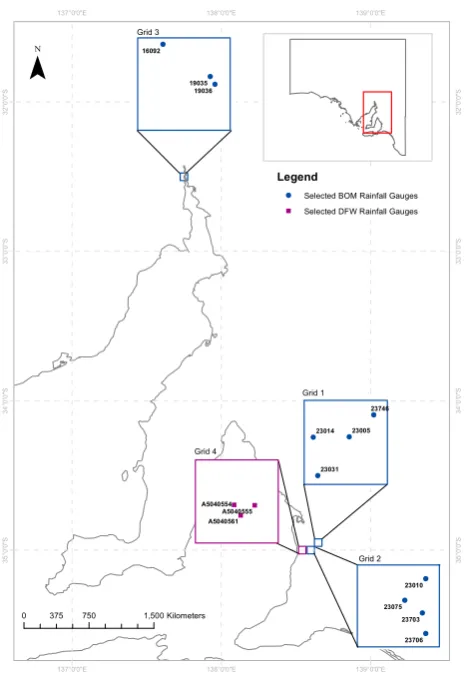
one gauge is likely to be different to the rainfall recorded at another gauge within the grid cell. To investigate this, three grid cells in SA which contain multiple BOM rainfall gauges and one grid cell that contains multiple DFW gauges (with overlapping records) were selected (see Fig. 3). Box and whisker plots of the annual rainfall for each gridded dataset and each gauge within the selected grid cells were then pro-duced and assessed.

3.3 Hydrological modelling implications

To investigate the hydrological modelling implications of us-ing gridded rainfall data as a surrogate for gauged data, a simple rainfall runoff model was developed. This modelling exercise aimed to highlight the sensitivities of hydrological modelling to changes in the rainfall input and therefore the potential issues associated with using gridded data for such an application. A daily rainfall-runoff model was developed using SIMHYD (i.e. the SIMple HYDrology model) for the upper Finniss River catchment in SA (Fig. 2). The catch-ment has an area of 192 km2 and fits within 13 grid cells. SIMHYD is a daily rainfall-runoff model which uses daily rainfall and areal potential evapotranspiration data to esti-mate daily stream flow. The model estiesti-mates runoff gener-ation from three sources: infiltrgener-ation excess runoff, interflow (and saturation excess runoff) and baseflow through the opti-misation of nine model parameters (refer to Peel et al., 2000, for further information on SIMHYD).

The model was initially calibrated for the period 1970 to 1986 and verified from 1987 to 2002 using gauged daily rain-fall data from BOM gauge 23808. A reasonable calibration was obtained, noting that natural streamflow data is partic-ularly difficult to obtain for SA due to diversions, extrac-tions and interbasin transfers (B. Murdoch, personal com-munication, 22 September 2010) with the monthly NSE val-ues achieved for the calibration and verification periods were 0.89 and 0.85 respectively. Following calibration and verifi-cation of the model and the resulting simulation of flow from 1970 to 2002 (i.e. the extent of the gauged daily rainfall data at gauge 23808) using gauged rainfall data, flow was also simulated for the period 1970 to 2009 using (i) AWAP daily gridded rainfall extracted at the gauge location, and (ii) SILO daily gridded rainfall extracted at the gauge location. The BOM gridded dataset was excluded from this analysis as daily data was not available. The SIMHYD model was then recalibrated using the AWAP daily gridded rainfall data and the resulting simulated flow compared with flows simulated using the gauged calibrated model. Monthly NSE values of 0.90 and 0.87 respectively, were achieved for the calibration and verification of this model. The calibration process was repeated again using SILO daily gridded rainfall with result-ing NSE values of 0.92 for the calibration period and 0.88 for the verification.

139°0'0"E 139°0'0"E

138°0'0"E 138°0'0"E

137°0'0"E 137°0'0"E

32

°0

'0

"S

32

°0

'0

"S

33

°0

'0

"S

33

°0

'0

"S

34

°0

'0

"S

34

°0

'0

"S

35

°0

'0

"S

35

°0

'0

"S

¯

0 375 750 1,500Kilometers

Grid 1

Grid 2 Grid 3

Grid 4 !

! ! 19035

19036 16092

! !

! ! 23746

23031 23014 23005

!

!

! ! 23010

23706 23703 23075

" "

" A5040561

A5040555 A5040554

Legend

! Selected BOM Rainfall Gauges

" Selected DFW Rainfall Gauges

Fig. 3. Location of selected grids in SA which encompass multiple

BOM (Grids 1, 2 and 3) and DFW (Grid 4) rainfall gauges.

4 Results

4.1 Intercomparison of gridded rainfall datasets

Fig. 4. (a) Annual average rainfall (1900–2008) for the AWAP gridded dataset. (b) Percentage difference in annual average rainfall (1900–

2008) between the SILO and AWAP datasets. (c) Percentage difference in annual average rainfall (1900–2008) between the BOM and AWAP datasets. (d) Percentage difference in annual rainfall totals between SILO and AWAP for 1900, 1930, 1960 and 1990. (e) Percentage difference in annual rainfall totals between BOM and AWAP for 1900, 1930, 1960 and 1990.

for most of the state except for small regions in the north, east and west. Again, the greater differences appear to be in areas of low gauge density. Overall, Fig. 4b and c confirm that the three gridded datasets are indeed different for SA.

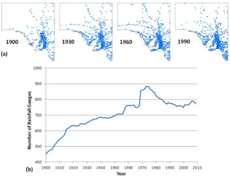
To explore the time variability of the results, the percent-age difference in annual rainfall totals between SILO and AWAP (Fig. 4d) and BOM and AWAP (Fig. 4e) at four points in time (i.e. 1900, 1930, 1960 and 1990) were determined. These points in time were chosen as they are representative

of different periods within the evolution of gauge density and distribution, illustrated by Fig. 5a, which indicates the spatial distribution of the BOM rainfall gauges in 1900, 1930, 1960 and 1990 and Fig. 5b, which shows changes in the number of BOM rainfall gauges in SA from 1900 to 2009.

The results clearly show that the differences between SILO and AWAP (Fig. 4d) and BOM and AWAP (Fig. 4e) vary across the four years. Reviewing the differences be-tween SILO and AWAP (Fig. 4d) in relation to Fig. 5a and

Fig. 5. (a) Indication of the number of rainfall gauges open in South

Australia in 1900, 1930, 1960 and 1990. (b) Evolution of rainfall gauges in South Australia from 1900 to 2009.

b, there does not appear to be an obvious reduction over time in the differences in areas where there has been an in-crease in the number of gauges (e.g. the southern third of the state). Similarly, Fig. 4d shows large differences that vary markedly over time between the SILO and AWAP datasets in the northern half of the state where there has been min-imal changes to gauge density. This suggests that the dif-ferences between the AWAP and SILO datasets are mainly due to differences in the methodologies used to create both datasets, rather than changes in gauge density and distribu-tion. Nevertheless it is still probable that changes to gauge quality and density contribute in some way to the observed differences between SILO and AWAP and further investiga-tion is required to definitively quantify this.

In regards to BOM and AWAP, it appears that the dif-ferences between the two datasets are greater in the north-ern half of the state (with differences ranging from less than

−50 % to greater than 50 %) compared with the southern half of the state (differences between−10 % and 5 %), where the majority of gauges are located. Reviewing the differences be-tween BOM and AWAP (Fig. 4e) in relation to Fig. 5a and b, it is clear that increases to gauge density is related to a de-crease in the differences between the two datasets. This result suggests that the differences between the BOM and AWAP gridded datasets are related to both differences in methodol-ogy used to develop the datasets and gauge density and dis-tribution.

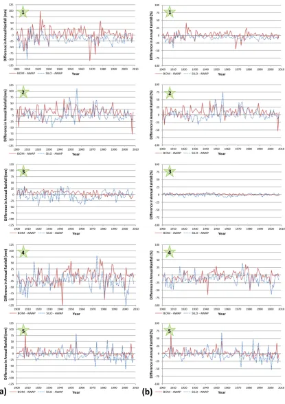
Figure 6a and b compare the three gridded datasets at five randomly selected ungauged points in SA (see Fig. 1 for point locations). Figure 6a shows the difference (in mm) be-tween annual totals for each gridded dataset extracted at each ungauged location and Fig. 6b shows the differences between annual rainfall totals as a percentage of AWAP annual aver-age rainfall for SILO and AWAP and BOM and AWAP. From

Fig. 6 it can be seen that the differences across the three grid-ded datasets vary. The percentage differences between the three datasets at point three are relatively small whereas at other points the differences in annual rainfall are quite large, ranging between−60 % and 75 %. Referring to the locations of the five random points shown in Fig. 1, it is evident that point 3 is closer to more BOM gauges relative to the other four ungauged locations. This may be a reason for the lower differences between the three gridded datasets at this point. It should be noted that there is no way of telling which of the gridded datasets is most representative of the real rainfall data at each of these points, since the random points were deliberately chosen so as not to overlap with an observation gauge. It is clear that for the selected locations, the three grid-ded datasets (BOM, SILO, AWAP) rarely agree (i.e. the lines indicating the level of difference in Fig. 6a and b rarely co-incide with zero). Importantly, there does not seem to be any systematic pattern to the disagreement (i.e. the differences appear to be random), though as mentioned gauge density could play a role. This raises the questions, what is the true rainfall timeseries at the chosen point since 1900? Which (if any) of the gridded datasets is a suitable representation of the observed data, which itself is an approximation of the actual climate conditions?

4.2 Comparison of gridded rainfall datasets against

gauged rainfall

4.2.1 Annual rainfall totals

The RMSE for each gridded data product as a percentage of annual gauged data as well as the annual average rainfall for each gauge are presented as a percentage of the annual gauge mean in Table 2. Note that the analyses have been undertaken for the period over which the gauged data commences and ceases (indicated in Table 1 for each gauge) or up to 2008 (when the BOM gridded data ceases).

37

-100 -75 -50 -25 0 25 50 75 100

1900 1910 1920 1930 1940 1950 1960 1970 1980 1990 2000 2010

Di

ffe

re

nc

e

in

A

nn

ua

l R

ai

nfa

ll

(%

)

Year

BOM - AWAP SILO - AWAP -125

-100 -75 -50 -25 0 25 50 75 100 125

1900 1910 1920 1930 1940 1950 1960 1970 1980 1990 2000 2010

Di

ffe

re

nc

e

in

A

nn

ua

l R

ai

nfa

ll

(m

m

)

Year

BOM - AWAP SILO - AWAP

-100 -75 -50 -25 0 25 50 75 100

1900 1910 1920 1930 1940 1950 1960 1970 1980 1990 2000 2010

Di

ffe

re

nc

e

in

A

nn

ua

l R

ai

nfa

ll

(%

)

Year

BOM - AWAP SILO - AWAP -125

-100 -75 -50 -25 0 25 50 75 100 125

1900 1910 1920 1930 1940 1950 1960 1970 1980 1990 2000 2010

Di

ffe

re

nc

e

in

A

nn

ua

l R

ai

nfa

ll

(m

m

)

Year

BOM - AWAP SILO - AWAP

4 4

5 5

-125 -100 -75 -50 -25 0 25 50 75 100 125

1900 1910 1920 1930 1940 1950 1960 1970 1980 1990 2000 2010

D

iff

er

en

ce

in

A

nn

ua

l R

ai

nfa

ll

(m

m

)

Year

BOM - AWAP SILO - AWAP

-100 -75 -50 -25 0 25 50 75 100

1900 1910 1920 1930 1940 1950 1960 1970 1980 1990 2000 2010

Di

ffe

re

nc

e

in

A

nn

ua

l R

ai

nfa

ll

(%

)

Year

BOM - AWAP SILO - AWAP -125

-100 -75 -50 -25 0 25 50 75 100 125

1900 1910 1920 1930 1940 1950 1960 1970 1980 1990 2000 2010

Di

ffe

re

nc

e

in

A

nn

ua

l R

ai

nfa

ll

(m

m

)

Year

BOM - AWAP SILO - AWAP

-100 -75 -50 -25 0 25 50 75 100

1900 1910 1920 1930 1940 1950 1960 1970 1980 1990 2000 2010

Di

ffe

re

nc

e

in

A

nn

ua

l R

ai

nfa

ll

(%

)

Year

BOM - AWAP SILO - AWAP -125

-100 -75 -50 -25 0 25 50 75 100 125

1900 1910 1920 1930 1940 1950 1960 1970 1980 1990 2000 2010

Di

ffe

re

nce

in

A

nn

ua

l R

ai

nfa

ll

(m

m

)

Year

BOM - AWAP SILO - AWAP

-100 -75 -50 -25 0 25 50 75 100

1900 1910 1920 1930 1940 1950 1960 1970 1980 1990 2000 2010

Di

ffe

re

nc

e

in

A

nn

ua

l R

ai

nfa

ll

(%

)

Year

BOM - AWAP SILO - AWAP

1 1

2 2

3 3

1

Figure 6. (a) Difference in annual rainfall totals between SILO and AWAP and BOM and

2

AWAP datasets at five random locations (marked 1, 2, 3, 4 and 5) in SA. (b) Difference

3

between annual rainfall totals as a percentage of AWAP annual average rainfall for SILO and

4

AWAP and BOM and AWAP datasets at five random locations in SA.

5

(b)

(a)

Fig. 6. (a) Difference in annual rainfall totals between SILO and AWAP and BOM and AWAP datasets at five random locations (marked 1,

2, 3, 4 and 5) in SA. (b) Difference between annual rainfall totals as a percentage of AWAP annual average rainfall for SILO and AWAP and BOM and AWAP datasets at five random locations in SA.

Table 2. Annual average rainfall for each gauge and the

correspond-ing annual Root Mean Square Error (RMSE) for each gridded data product in mm and (in brackets) as a percentage of annual gauged data. Gray highlighted cells indicate the closest match to gauged.

Gauged

Gauge annual average Annual RMSE mm (%)

No. rainfall (mm) BOM SILO AWAP

16031 178.6 16.1 (9.0) 1.8 (1.0) 25.9 (14.5)

16055∗ _{273.7 45.5 (16.6) 4.3 (1.6) 23.8 (8.7)}

16083∗ 158.4 38.8 (24.5) 21.8 (13.8) 46.3 (29.2)

17052 167.4 25.5 (15.2) 26.4 (15.7) 34.0 (20.3)

17125 171.0 35.1 (20.5) 25.3 (14.8) 39.5 (23.1)

17132 118.0 8.2 (6.9) 3.8 (3.2) 14.4 (12.2)

18069∗ 431.2 29.6 (6.9) 7.7 (1.8) 35.9 (8.3)

18146 192.3 46.2 (24.0) 2.7 (1.4) 20.1 (10.5)

19001∗ 385.4 46.6 (12.1) 10.2 (2.7) 63.3 (16.4)

19047 316.5 32.2 (10.2) 10.5 (3.3) 35.0 (11.0)

20050 241.9 67.9 (28.1) 2.8 (1.2) 68.8 (28.4)

21027 465.0 44.6 (9.6) 24.5 (5.3) 36.1 (7.8)

23318 545.8 40.2 (7.4) 34.3 (6.3) 41.8 (7.6)

23721∗ _{639.1 54.1 (8.5) 43.8 (6.9) 52.9 (8.3)}

23736 1180.3 218.3 (18.5) 170.6 (14.5) 230.7 (19.5)

23808 856.0 80.5 (9.4) 7.3 (0.8) 57.2 (6.7)

A4260638 613.4 111.3 (18.1) 49.4 (8.1) 174.0 (28.4)

A4260639 759.3 41.3 (5.4) 48.0 (6.3) 50.7 (6.7)

A5040552 1068.5 91.2 (8.5) 90.8 (8.5) 80.3 (7.5)

A5040558 660.2 74.6 (11.3) 175.8 (26.6) 107.9 (16.3)

A5040559 848.3 74.9 (8.8) 101.9 (12.0) 79.9 (9.4)

A5050502 496.2 28.6 (5.8) 72.8 (14.7) 24.7 (5.0)

A5060500 440.7 83.0 (18.8) 33.8 (7.7) 79.3 (18.0)

A5080504 501.4 47.1 (9.4) 43.6 (8.7) 39.8 (7.9)

A5100516 193.2 23.9 (12.4) 65.9 (34.1) 29.6 (15.3)

A5130505 685.8 156.3 (22.8) 155.6 (22.7) 153.8 (22.4)

4.2.2 Annual rainfall in grid cells with multiple gauges

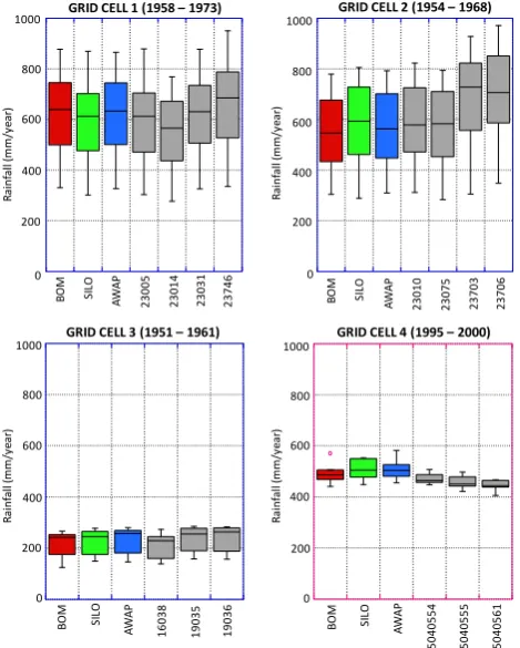
Figure 3 shows the location of the four SA grid cells and the gauges within each grid cell that were investigated. These grid cells were selected as they contain several rain-fall gauges with overlapping records. Note that each grid cell was analysed over a different time period (indicated in Fig. 7) with the periods selected to maximise the number of overlap-ping gauged records. Figure 7 shows box and whisker plots of the annual rainfall recorded at each gauge and the corre-sponding gridded rainfall data for the same time period for the grid cell within which the gauges sit. Note that each box represents 50 % of the data and the median value is indi-cated by the line through the box. The lines that extend from the box represent the minimum and maximum values within the dataset that fall within an acceptable range (typically 1.5 times the width of the box). Circles (only seen in grid cell 4 in Fig. 7) represent values outside the acceptable range (i.e. outliers in the dataset).

The large range in annual rainfall that occurs in a sin-gle grid cell is evident in Fig. 7, particularly in grid cell 1, where the maximum annual totals for the gauges range from the maximum of 770 mm at gauge 23014 to the max-imum of 950 mm recorded at gauge 23746. This highlights the short range spatial correlation of rainfall (e.g. Jeffrey et al., 2001) and the flaw in assuming that gridded rainfall is

representative of rain everywhere within a given grid cell. Conversely, it could also suggest that gauged rainfall cannot adequately represent rainfall over a grid cell.

It is evident that the rainfall range of the gridded datasets does not fully encompass the gauged range (for both the BOM and DFW gauges) and therefore does not capture the highs and lows of the gauged rainfall data. It would appear, particularly for Grids 2 and 4, that the gridded datasets tend to capture the midpoint of the gauged data. This is perhaps no surprise in regards to the BOM and AWAP datasets given that the methods used to create these datasets aim to capture the areal average (Jones and Weymouth, 1997). Of particular interest is that although the SILO interpolation method is set to exactly interpolate the gauged data (Jeffrey et al., 2001), as evident from the Fig. 7, it is obviously not possible for the SILO method to match the data exactly at all locations simultaneously, especially non-BOM gauges. Ultimately the results of this analysis indicate that the gridded datasets do not accurately capture the spatial variability within a grid cell or, in most cases, the gauged wet and dry extremes. This is further analysed in the following sections.

4.2.3 Seasonal rainfall totals

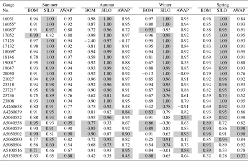
The seasonal NSE values calculated in the comparison of the gridded and gauged datasets at each BOM and DFW gauge selected are presented in Table 3. As with the annual anal-yses (discussed in Sect. 4.2.1), the seasonal analanal-yses have been undertaken for the period over which the gauged data commences and ceases (indicated in Table 1 for each gauge) or up to 2008 (when the BOM gridded data ceases).

38

0 200 400 600 800 1000

BOM SILO AWAP 23010 23075 23703 23706 GRID 2

Ra

inf

al

l

(m

m

/y

ea

r)

0 200 400 600 800 1000

BOM SILO AWAP 23005 23014 23031 23746 GRID 1

Ra

inf

al

l

(m

m

/y

ea

r)

GRID CELL 1 (1958 – 1973) 1000

600 800

200 400

0

B

O

M

SI

LO

A

W

A

P

23005 23014 23031 23746

R

ai

nf

al

l (

m

m

/y

ear

)

1000

600 800

200 400

0

GRID CELL 2 (1954 – 1968)

R

ai

nf

al

l (

m

m

/y

ear

)

B

O

M

SI

LO

A

W

A

P

23010 23075 23703 23706

1

0 200 400 600 800 1000

BOM SILO AWAP 16038 19035 19036 GRID 8_UpdatedMarch2012

Ra

n

ge

GRID CELL 3 (1951 – 1961)

B

O

M

SI

LO

A

W

A

P

16038 19035 19036

R

ai

nf

al

l (

m

m

/y

ear

)

R

ai

nf

al

l (

m

m

/y

ear

)

B

O

M

SI

LO

A

W

A

P

A

5

0

4

0

5

5

4

GRID CELL 4 (1995 – 2000) 1000

600 800

200 400

0

1000

600 800

200 400

00 200 400 600 800 1000

BOM SILO AWAP A5040554 A5040555 A5040561 DFW Grid

Ra

n

ge

A

5

0

4

0

5

5

5

A

5

0

4

0

5

6

1

2

Figure 7. A comparison of annual BOM (red boxes), SILO (green boxes) and AWAP (blue 3

boxes) gridded rainfall data and gauged (grey boxes) annual rainfall data in four grid cells in 4

SA. Note that grid cells 1, 2, and 3 feature only BOM gauges and grid cell 4 includes only 5

DFW gauges. The time period over which the analysis was undertaken is given in the figure. 6

Fig. 7. A comparison of annual BOM (red boxes), SILO (green

boxes) and AWAP (blue boxes) gridded rainfall data and gauged (grey boxes) annual rainfall data in four grid cells in SA. Note that grid cells 1, 2, and 3 feature only BOM gauges and grid cell 4 in-cludes only DFW gauges. The time period over which the analysis was undertaken is given in the figure.

In contrast to these results the seasonal NSE values cal-culated in the comparison of the gridded datasets and DFW gauges are much more scattered, which is made obvious by the scattering of green cells (i.e. cells that indicate the high-est NSE value determined for that gauge). It is evident that none of the gridded datasets match (i.e. records a high NSE value) the DFW gauged data consistently. Of interest is that for all seasons, the NSE values recorded for the SILO dataset for DFW gauges ranges from−0.30 to 0.96 whereas for the BOM gauges this range is 0.73 to 1.00, with the majority of NSE values around 1.00. This result supports the findings of Sect. 4.2.1 and suggests that the performance of SILO in mimicking observed data at non-BOM gauges is variable (i.e. the performance of SILO depends on which gauged data it is fitted to).

The under-representation of high elevation areas in gaug-ing networks is a known cause of interpolation errors (Jef-frey et al., 2001; Beesley et al., 2009) and may explain the poor annual RMSE and seasonal NSE results obtained at high elevation gauge 23736. To investigate the performance of gridded data in relation to elevation, seasonal NSE values

calculated for each gauge for each gridded dataset were plot-ted against gauge elevation. The results for each season are shown in Fig. 8 with the seasonal NSEs calculated for BOM gauges in the left column and NSEs determined for the DFW gauges in the right column. Initially referring only to the BOM gauges, it is evident that the values determined for SILO for all seasons congregate around an NSE value of 1, whereas the values determined for AWAP and BOM tend to be much more scattered. There is no obvious trend in NSE value and elevation; however there is a clear outlier, which corresponds again to the highest gauge, 23736 (elevation 727 mAHD). All three data sets perform relatively poorly at this location in all seasons. However, it is unclear from this analysis whether the high elevation, and associated low gauge density, is responsible for the low NSE values at this site, or the fact that the gauge record ceases in 1956. In any case, it is clear that issues associated with temporal and spa-tial completeness (i.e. gauge density, e.g. Jones and Trewin, 2000) and the impact that has on the accuracy of gridded datasets needs further investigation and quantification.

The increase in the range of NSE values obtained for SILO for the DFW gauges relative to the BOM gauge results (men-tioned earlier) is clearly evident in Fig. 8. There is no obvious pattern in seasonal NSE value and elevation (e.g. an increase in elevation does not necessarily result in a decrease in NSE value as one might expect), with NSE values for all grid-ded datasets for the DFW gauges very scattered in all sea-sons. Of note, however, are the relatively high NSE values recorded for all seasons and all gridded datasets for the high-est elevation DFW gauge (A5040552, 686 mAHD). This re-sult may give weight to the suggestion that the low NSE val-ues recorded for the highest elevation BOM gauge (23736) may be due to the fact that the gauge record ceases in 1956 rather than the high elevation. Although an interesting result, further assessment of high elevation gauges (of which SA has very few) is required to substantiate this observation. Never-theless, the key result from this analysis is that there is no obvious seasonal pattern to the differences between the grid-ded and gauged datasets.

4.2.4 Monthly rainfall extremes

An important aspect required of gridded data is the ability to capture high and low rainfall extremes, since it is often the extremes that are of interest in hydrological, climatological, and agricultural studies. To explore this issue further, Table 4 indicates both the number of months with less than 1 mm (i.e. “no rainfall” months) recorded by each data product and the number of months (for each data product) that are greater than the gauged 99th percentile rainfall. Note that the gauged 99th percentile rainfall is provided in brackets in Table 4. To complement this information, Table 5 indicates the total ac-cumulated rainfall (in mm) for each dataset that corresponds to the number of gauged “no rain” months, and the total rain-fall (in mm) for each dataset that corresponds to the number

0 100 200 300 400 500 600 700 800

0 0.1 0.2 0.3 0.4 0.5 0.6 0.7 0.8 0.9 1

El

e

va

ti

o

n

(m

A

HD

)

Nash Sutcliffe Efficiency

BOM SILO AWAP

0 100 200 300 400 500 600 700 800

0 0.1 0.2 0.3 0.4 0.5 0.6 0.7 0.8 0.9 1

El

e

va

ti

o

n

(m

A

HD

)

Nash Sutcliffe Efficiency

BOM SILO AWAP

0 100 200 300 400 500 600 700 800

El

e

va

ti

o

n

(m

A

HD

)

Nash Sutcliffe Efficiency

BOM SILO AWAP

0 100 200 300 400 500 600 700 800

0 0.1 0.2 0.3 0.4 0.5 0.6 0.7 0.8 0.9 1

El

e

va

ti

o

n

(m

A

HD

)

Nash Sutcliffe Efficiency

BOM SILO AWAP

0 100 200 300 400 500 600 700 800

-0.2 -0.1 0 0.1 0.2 0.3 0.4 0.5 0.6 0.7 0.8 0.9 1

El

e

va

ti

o

n

(m

A

HD

)

Nash Sutcliffe Efficiency

BOM SILO AWAP

0 100 200 300 400 500 600 700 800

El

e

va

ti

o

n

(m

A

HD

)

Nash Sutcliffe Efficiency BOM SILO AWAP

0 100 200 300 400 500 600 700 800

0 0.1 0.2 0.3 0.4 0.5 0.6 0.7 0.8 0.9 1

El

e

va

ti

o

n

(m

A

HD

)

Nash Sutcliffe Efficiency

BOM SILO AWAP

0 100 200 300 400 500 600 700 800

0 0.1 0.2 0.3 0.4 0.5 0.6 0.7 0.8 0.9 1

El

e

va

ti

o

n

(m

A

HD

)

Nash Sutcliffe Efficiency

BOM SILO AWAP

Summer (Dec-Jan-Feb)

Autumn (Mar-Apr-May)

Winter (Jun-Jul-Aug)

Spring (Sep-Oct-Nov)

BOM Gauges

BOM Gauges

BOM Gauges

DFW Gauges

DFW Gauges

DFW Gauges

DFW Gauges

1

Figure 8. Comparison of seasonal NSE values and elevation for (a) Bureau of Meteorology

2

(BOM) gauges and (b) Department for Water (DFW) gauges .

3

(a)

(b)

Fig. 8. Comparison of seasonal NSE values and elevation for (a) Bureau of Meteorology (BOM) gauges and (b) Department for Water

Table 3. Seasonal NSE values of gridded vs gauged data. Gray highlighted cells indicate the closest match to gauged.

Gauge Summer Autumn Winter Spring

No. BOM SILO AWAP BOM SILO AWAP BOM SILO AWAP BOM SILO AWAP

16031 0.94 1.00 0.93 0.98 1.00 0.95 0.97 1.00 0.95 0.96 1.00 0.84 16055∗ 0.91 1.00 0.92 0.87 1.00 0.95 0.80 1.00 0.94 0.85 1.00 0.93 16083∗ 0.91 0.97 0.80 0.72 0.96 0.72 0.93 0.93 0.92 0.88 0.95 0.91 17052 0.90 0.82 0.80 0.98 1.00 0.97 0.96 0.98 0.92 0.95 1.00 0.95 17125 0.97 1.00 0.94 −2.40 0.97 −0.17 0.95 1.00 0.92 0.90 1.00 0.93 17132 0.98 1.00 0.92 0.81 1.00 0.91 0.95 1.00 0.84 0.83 1.00 0.91 18069∗ 0.94 1.00 0.92 0.94 0.99 0.92 0.94 1.00 0.92 0.94 1.00 0.95 18146 0.78 1.00 0.97 0.58 1.00 0.97 0.81 1.00 0.95 0.69 1.00 0.91 19001∗ 0.95 1.00 0.94 0.92 1.00 0.88 0.67 1.00 0.35 0.93 1.00 0.88 19047 0.93 0.99 0.94 0.93 0.99 0.92 0.88 0.99 0.85 0.94 0.99 0.93 20050 0.91 1.00 0.93 0.92 1.00 0.92 −0.13 1.00 −0.09 0.79 1.00 0.76 21027 0.94 0.99 0.93 0.96 0.98 0.97 0.85 0.96 0.91 0.92 0.98 0.92 23318 0.94 0.98 0.94 0.92 0.96 0.93 0.94 0.95 0.93 0.94 0.98 0.93 23721∗ 0.95 0.98 0.96 0.90 0.96 0.91 0.87 0.94 0.88 0.82 0.95 0.93 23736 0.75 0.89 0.76 0.62 0.81 0.62 0.67 0.76 0.61 0.59 0.73 0.52 23808 0.93 1.00 0.94 0.90 1.00 0.95 0.69 1.00 0.79 0.94 1.00 0.95 A4260638 0.80 0.91 0.77 0.73 0.92 0.48 0.42 0.78 −0.91 0.69 0.92 0.33 A4260639 0.91 0.95 0.91 0.81 0.82 0.84 0.83 0.79 0.82 0.93 0.95 0.86 A5040552 0.88 0.94 0.88 0.93 0.96 0.95 0.91 0.88 0.93 0.89 0.92 0.90 A5040558 0.95 0.93 0.95 0.77 0.33 0.67 0.86 −0.30 0.63 0.89 0.72 0.82 A5040559 0.90 0.91 0.90 0.95 0.92 0.92 0.89 0.82 0.83 0.90 0.86 0.90 A5050502 0.90 0.81 0.90 0.90 0.87 0.90 0.91 0.63 0.93 0.98 0.91 0.98 A5060500 0.77 0.85 0.82 0.72 0.93 0.82 0.25 0.91 0.17 0.85 0.94 0.84 A5080504 0.56 0.60 0.54 0.68 0.73 0.72 0.54 0.74 0.73 0.93 0.89 0.92 A5100516 0.71 0.66 0.67 0.91 0.93 0.95 0.84 −0.01 0.88 0.89 0.33 0.78 A5130505 0.63 0.65 0.68 0.42 0.35 0.45 0.68 0.65 0.64 0.32 0.28 0.37

of gauged months that are greater than the gauged 99th per-centile rainfall. For example, Table 4 indicates that there are 187 recorded “no rain” months at BOM gauge 16031. The gauged rainfall accumulation of these 187 months is 13.7 mm (Table 5), whereas for the same months, the AWAP, BOM and SILO accumulations are 98.7 mm, 85.0 mm and 14.1 mm respectively. Note that where there is more than one green cell highlighted in Tables 4 and 5, it indicates that more than one of the gridded datasets was closest to the gauged result.

In regards to the “no rain” months, if the gridded dataset underestimates the number of gauged “no rain” months, it suggests that the interpolation process is not capturing the gauged dry periods. This appears to be the case for 13 of the 16 BOM gauges where the number of “no rain” months recorded for the BOM and AWAP gridded datasets underes-timates the number of gauged “no rain” months. SILO more closely matches the number of gauged “no rain” months but there are still some marked differences. The implications of this are clear from Table 5 where it is shown that all gridded datasets (except for SILO at gauge 19001 and 23808) over-estimate the level of rainfall recorded at each location dur-ing months observed to have “no rain”. In some cases, the overestimation is significant. For example, for gauge 16083, SILO overestimates the gauged rainfall recorded in “no rain”

months by approximately 15 times and BOM and AWAP overestimate by 49 and 56 times respectively. For gauge 17052 the overestimation is even higher for BOM and AWAP. BOM and AWAP record similar accumulations for all gauges except 18146 where BOM overestimates the gauged accumu-lations by approximately 100 times and AWAP a relatively low 20 times. There is no obvious reason for this discrepancy. The results for the DFW gauges again appear a lot more variable. At 7 of the 10 DFW gauges, the three grid-ded datasets reasonably match the gauged accumulation. However, for the remaining three gauges (i.e. A4260639, A5100516 and A5130505), the overestimation is substan-tial. For example, for DFW gauge A5130505, BOM overes-timates the gauged “no rain” accumulation by approximately 400 times, and AWAP and SILO overestimate by approxi-mately 435 and 470 times respectively. Overall, these results, particularly the BOM gauge results, indicate that the grid-ded datasets tend to overestimate the dry gauged periods and there does not appear to be any systematic pattern to the over-estimations.

On the other end of the scale, if the gridded dataset un-derestimates the number of months greater than the gauged 99th percentile rainfall, it suggests that the interpolation method underestimates the wet periods. Table 4 shows that in

Table 4. Number of months with<1 mm rainfall (“no rain” months) and the number of months>the gauged 99th percentile rainfall (with the gauged 99th percentile rainfall given in brackets). Gray highlighted cells indicate the closest match to gauged.

Number of “no rain” months Number of months>gauged

Gauge 99th percentile rainfall

No. Gauged BOM SILO AWAP Gauged BOM SILO AWAP

16031 187 176 188 173 9 (90.1) 7 10 9

16055* 120 88 121 83 14 (97.4) 6 13 9

16083* 566 494 594 454 14 (120.3) 14 14 20

17052 456 257 454 314 12 (140.6) 11 12 7

17125 52 44 53 45 2 (107.4) 1 2 2

17132 46 40 46 39 2 (88.0) 2 2 2

18069* 55 57 58 68 14 (133.8) 11 15 11

18146 62 22 62 53 4 (100.2) 2 4 3

19001* 63 39 64 45 14 (115.6) 16 12 21

19047 106 74 112 78 13 (103.3) 15 13 17

20050 97 64 97 63 5 (140.9) 6 5 6

21027 45 42 51 41 14 (132.2) 8 13 9

23318 42 39 38 38 14 (143.9) 6 15 5

23721* 22 17 25 19 14 (169.7) 20 8 17

23736 6 8 10 3 6 (330.6) 2 3 1

23808 2 2 2 2 4 (203.4) 4 4 3

A4260638 2 2 4 2 2 (166.4) 7 5 13

A4260639 5 2 2 1 3 (185.2) 2 1 2

A5040552 1 2 2 2 3 (277.6) 2 3 2

A5040558 3 3 2 3 3 (216.9) 4 8 5

A5040559 3 3 4 3 3 (241.3) 1 5 1

A5050502 9 7 10 7 3 (126.0) 4 1 4

A5060500 9 7 10 8 3 (113.8) 6 2 7

A5080504 8 6 10 8 3 (137.6) 4 3 2

A5100516 56 41 33 46 3 (101.7) 3 4 4

A5130505 9 3 3 1 3 (206.3) 0 1 0

general, the number of months greater than the gauged 99th percentile recorded for each gridded dataset is close to the number of gauged months (for both BOM and DFW gauges) greater than the gauged 99th percentile rainfall. However, when looking at the accumulated rainfall in these months some key differences emerge. Table 5 indicates that for months where the BOM gauged rainfall was greater than the gauged 99th percentile SILO and BOM gridded datasets un-derestimate the gauged accumulated rainfall at 14 of the 16 gauges, and AWAP, 12 of the 16 gauges. Importantly, when compared to the annual average rainfall at each of the BOM gauges (Table 2), the underestimations are highly significant amounts.

Again the results for the DFW gauges are more variable, with all gridded datasets underestimating the gauged accu-mulation at 6 of the 10 gauges, but not necessarily the same gauges. For the remaining 4 gauges, the gridded datasets overestimate the gauged accumulations.

Ultimately, these results demonstrate that in addition to overestimating the amount of rainfall that occurs during dry (i.e.<1 mm monthly rainfall) conditions the gridded datasets

also tend to underestimate the amount of rainfall that occurs when it is extremely wet.

These results are in line with the findings of Beesley et al. (2009) who, in their review of daily AWAP and SILO er-ror statistics, found that there is a negative/positive bias in the gridded datasets for higher/lower rainfall areas. Similar results were found by Silva et al. (2007) and Ensor and Robe-son (2008) in their compariRobe-sons of gridded and gauged data in Brazil and Midwestern USA respectively, which indicates that the “smoothing out” of extreme rainfall events is a com-mon issue with gridded datasets.

5 Implications of using gridded rainfall data as a

surrogate for observed in hydrological modelling

Table 5. Rainfall accumulation during gauged “no rain” months and gauged months greater than the gauged 99th percentile. Gray highlighted

cells indicate the closest match to gauged.

Total rainfall (in mm) corresponding Total rainfall (in mm) corresponding to gauged “no rain” months to the number of gauged months>

gauged 99th percentile rainfall Gauge No. Gauged BOM SILO AWAP Gauged BOM SILO AWAP 16031 13.7 85.0 14.1 98.7 987.6 922.8 979.7 875.6 16055* 13.5 113.7 18.5 112.3 1673.6 1315.6 1643.4 1429.2 16083* 13.1 647.7 204.9 735.3 3008.0 2680.0 2936.4 2561.1 17052 9.6 730.3 100.9 577.1 2242.2 2046.2 1989.1 1817.9 17125 2.6 44.1 2.9 38.4 258.5 248.6 255.7 264.9 17132 3.8 32.0 4.3 33.7 209.8 209.3 206.2 246.2 18069* 12.8 40.2 17.9 22.4 2156.7 2022.1 2138.5 2030.2 18146 2.4 250.5 2.6 48.5 597.8 390.7 591.3 551.3 19001* 15.4 71.1 14.3 58.9 1777.1 1776.2 1749.1 1815.2 19047 12.5 130.0 16.7 115.8 1623.0 1442.7 1556.9 1395.9 20050 5.4 138.0 5.5 123.6 847.1 885.1 840.5 892.6 21027 11.4 34.2 18.7 32.0 2049.8 1781.7 1953.4 1837.2 23318 7.4 29.7 14.3 30.8 2279.8 2082.7 2311.6 2063.3 23721* 7.5 24.5 9.1 18.1 2652.1 2664.2 2584.1 2595.8 23736 2.1 69.1 67.7 68.4 2285.5 1889.8 1923.5 1754.4

23808 0 1.4 0 0.4 943.5 825.3 944.5 863.3

A4260638 0.8 1.6 0.0 1.2 380.7 434.1 400.5 466.8 A4260639 0.0 252.0 264.8 259.5 594.8 613.0 617.6 625.5 A5040552 0.2 0.0 0.0 0.0 915.8 775.0 825.7 770.0 A5040558 0.6 0.7 1.3 0.7 654.8 687.9 845.0 751.6 A5040559 1.4 2.5 1.6 2.0 825.0 744.1 807.6 699.2 A5050502 1.6 11.8 6.0 11.5 388.2 364.2 322.1 355.0 A5060500 1.2 6.1 1.0 4.0 386.0 406.3 360.1 418.5 A5080504 1.8 5.9 4.6 4.1 466.2 322.4 331.1 317.3 A5100516 6.9 175.9 163.2 128.0 436.0 435.9 471.9 425.6 A5130505 0.8 322.1 377.1 348.2 631.6 558.6 593.7 540.3

using AWAP and SILO as inputs ceases in 2009). It is ev-ident from Fig. 9 that the flow simulated using the AWAP gridded rainfall data for the model calibrated to gauged (blue line) tends not to reach the high flow extremes of the ob-served gauged flow (purple line) or the flow simulated using gauged rainfall data (red line). This is particularly obvious during the period 1985 to 1990. On the other end of the scale the low gauged flows tend to be overestimated by the AWAP simulated flow. The flow simulated using SILO data (green line) was a much closer match to observed gauge flow which was to be expected given results from Section 4 which show a closer agreement between SILO gridded rainfall data and BOM gauged rainfall.

It should also be noted, that from 1997 to 1999 the flow simulated using AWAP rainfall data for the model calibrated to gauged (blue line) is closer to the gauged flow relative to the flow simulated using gauged rainfall. This is a cu-rious result that we cannot explain other than to speculate that this period, which coincided with extreme drought con-ditions across south-east Australia (e.g. Verdon-Kidd and Kiem, 2009, 2010), may have been associated with diver-sions or extractions within the catchment that were not

properly accounted for in the “naturalised” flow record or were not adequately represented or parameterised in the cal-ibration period.

Also included in Fig. 9 is the flow simulated using AWAP rainfall and the SIMHYD model that was calibrated using AWAP rainfall (dashed orange line). The fact that this flow simulation is so different to the flow simulated with the same input data but a model calibrated on gauged data (blue line) reinforces the points made in Sect. 4 – that gridded rainfall data is different to gauged data. The implications of this are stark given the large differences in flow simulations (blue line versus dashed orange line) that are totally dependent on whether the hydrological model is calibrated using gauged or gridded data – again highlighting the point that gridded data is sometimes quite different to gauged data. Similar conclu-sions can be made if AWAP is replaced with SILO, as shown in Fig. 9.

Annual, seasonal and monthly NSE statistics for (1) AWAP rainfall data compared with gauged rainfall data (BOM gauge number 23808), (2) flow simulated using AWAP data and the gauged flow data (A4260504) (for the model calibrated to gauged rainfall) and (3) flow simulated