Towards model evaluation and identification using Self Organizing Maps

the Creative Commons Attribution 3.0 License.

Sciences

Towards model evaluation and identification using Self-Organizing

Maps

M. Herbst and M. C. Casper

Department of Physical Geography, University of Trier, Germany

Received: 17 October 2007 – Published in Hydrol. Earth Syst. Sci. Discuss.: 5 November 2007 Revised: 13 February 2008 – Accepted: 17 March 2008 – Published: 9 April 2008

Abstract. The reduction of information contained in model time series through the use of aggregating statistical perfor-mance measures is very high compared to the amount of in-formation that one would like to draw from it for model iden-tification and calibration purposes. It has been readily shown that this loss imposes important limitations on model identifi-cation and -diagnostics and thus constitutes an element of the overall model uncertainty. In this contribution we present an approach using a Self-Organizing Map (SOM) to circumvent the identifiability problem induced by the low discrimina-tory power of aggregating performance measures. Instead, a Self-Organizing Map is used to differentiate the spectrum of model realizations, obtained from Monte-Carlo simulations with a distributed conceptual watershed model, based on the recognition of different patterns in time series. Further, the SOM is used instead of a classical optimization algorithm to identify those model realizations among the Monte-Carlo simulation results that most closely approximate the pattern of the measured discharge time series. The results are an-alyzed and compared with the manually calibrated model as well as with the results of the Shuffled Complex Evo-lution algorithm (SCE-UA). In our study the latter slightly outperformed the SOM results. The SOM method, however, yields a set of equivalent model parameterizations and there-fore also allows for confining the parameter space to a region that closely represents a measured data set. This particular feature renders the SOM potentially useful for future model identification applications.

1 Introduction

Information from existing or additional observed sources is crucial to decrease model uncertainty. Model evaluation and model identification usually resort to aggregating statistical

Correspondence to: M. Herbst

([email protected])

al. (2000), Vrugt et al. (2003) and Wagener et al. (2004). Yet model identification methods that depend on common sta-tistical approaches might still not be able to extract enough information relevant to this task (Gupta et al., 2003). An ex-citing new point of view for model evaluation and identifica-tion that tackles these shortcomings emerges from the trans-formation of the existing data into the frequency domain and the wavelet domain (e.g. Clemen, 1999; Lane, 2007; Monta-nari and Toth, 2007).

In order to improve model identifiability (as proposed by Gupta et al., 1998; Yapo et al., 1998; Boyle et al., 2000) and the extraction of information from existing data we in-troduce an approach that, in a sense, emulates the visual as-sessment of model hydrographs. To circumvent the ambigu-ity induced by standard objective functions a Self-Organizing Map (SOM) (Kohonen, 2001) is used to represent the spec-trum of model realizations obtained from Monte-Carlo simu-lations with a distributed conceptual watershed model based on the recognition of different patterns of model residual time series.

Self-Organizing maps have found successful practical ap-plications in speech recognition, image analysis, catego-rization of electric brain signals (Kohonen, 2001) as well as process monitoring (Alhoniemi et al., 1999; Simula et al., 1999) and local time series modelling (Vesanto, 1997; Principe et al., 1998; Cho, 2004). Similarly diverse are the currently emerging applications of SOM in the field of hy-drology: Examples for the analysis of hydrochemical data can be found in Peeters et al. (2007) and Lischeid (2006). Sch¨utze et al. (2005) apply a variant of the SOM to approx-imate the Richards equation and its inverse solution. Hsu et al. (2002) successfully performed system identification and daily streamflow predictions with the Self-Organizing Lin-ear Output Mapping Network (SOLO). They used a SOM to control local regression functions according to the stage of the rainfall-runoff process. Kalteh and Berndtsson (2007) use SOM for the interpolation of monthly precipitation.

In Sect. 2.1 of this contribution we summarize the princi-ples and advantages of SOM and describe how this method is applied to yield a topologically ordered mapping of model output time series according to the similarity in the tempo-ral patterns of their residuals obtained through Monte-Carlo simulations. The properties of this “semantic map” of model realizations will be examined by relating the map elements (i) to the standard performance measures of the associated model runs and (ii) to the parameter values that have been used to generate the model results. It is shown that a SOM is capable of giving visual insights into the parameter sen-sitivity and the operating of the model structure. Moreover, in the second part of this article these properties are used to introduce an application of the Self-Organizing Map for parameter identification purposes. The SOM is used to iden-tify those model realizations among a given set of Monte-Carlo simulations results that most closely approximate the pattern of the measured time series, i.e. the “zero-residual”

realization. The result will be analyzed and compared with the manually calibrated model as well as with the result of the single-objective Shuffled Complex Evolution algorithm (SCE-UA, Duan et al., 1993).

2 Methods

2.1 The Self-Organizing Map

The Self-Organizing Map is a type of artificial neural net-work (ANN) and unsupervised learning algorithm that is used for clustering, visualization and abstraction of multi-dimensional data. Unlike other types of ANN it has no out-put function. Instead it maps vectorial inout-put data items with similar patterns onto contiguous locations of a discrete low-dimensional grid of neurons in a topology-preserving man-ner. Therefore its output can be compared to a semantic map: nearby locations on the map are attributed similar data pat-terns. Each of the map’s neurons becomes “sensitized” to a different domain of the patterns contained in the vectorial training data items, i.e. the map units act as decoder for dif-ferent types of patterns contained in the input data (Kohonen, 2001).

Each input data itemx∈Xis considered as a vector

x=[x1, x2, . . . , xn]T ∈ <n (1)

withnbeing the dimension of the input data space. A fixed number ofkneurons indexediis arranged on a regular grid

Gwith each neuron being associated to a weight vector

mi =[µi1, µi2, . . . , µin]T ∈ <n (2)

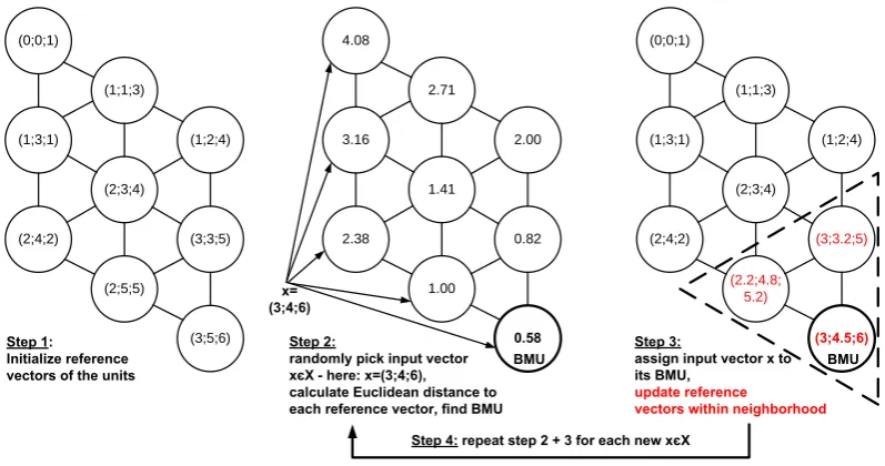
also called reference vector, which has the same dimen-sionality as the input vectorsx∈X. These weights connect each input vectorx in parallel to all neurons ofG. More-over the neurons are connected to each other. In our case this interconnection is defined on a hexagonal grid topology. The training of the SOM now comprises the following steps (Fig. 1):

1. The components of the mi are initialized with a se-quence of values from points on the plane spanned by the two greatest eigenvectors of the data distribution. This pro-cedure assures a faster and more reliable convergence of the algorithm (Kohonen, 2001).

2. Randomly pick an input vector samplex∈X and com-pute the Euclidean distance

kx−mik =

v u u t

n

X

j=1

xj−mij

2

(3)

betweenxand each of the reference vectorsmi(as a measure of similarity, generally any other metric can be applied as well) and find the neuron c(x) with a reference vectormc such that

kx−mck =min i

(0;0;1)

(1;1;3)

(1;2;4)

(2;3;4)

(3;3;5)

(2;5;5)

(3;5;6) (1;3;1)

(2;4;2)

4.08

2.71

2.00

1.41

0.82

1.00

0.58

3.16

2.38

Step 2:

randomly pick input vector xєX - here: x=(3;4;6),

calculate Euclidean distance to each reference vector, find BMU

(0;0;1)

(1;1;3)

(1;2;4)

(2;3;4)

(3;3.2;5)

(2.2;4.8; 5.2)

(3;4.5;6)

(1;3;1)

(2;4;2)

x= (3;4;6) Step 1:

Initialize reference vectors of the units

Step 3:

assign input vector x to its BMU,

update reference

vectors within neighborhood

Step 4: repeat step 2 + 3 for each new xєX

BMU BMU

Fig. 1. The basic steps of the SOM algorithm.

cis then called the best-matching unit (BMU) and defines the image of the samplexon the mapG.

3. The nodes that are within a certain distance of the “win-ning neuron”care updated according to the equation mi(t+1)=mi(t )+α (t ) hci(t )[x(t )−mi(t )] (5) wheret is the number of the iteration step andmi(t )is the current weight vector which is updated proportionally to the difference [x(t )−mi(t )]. hci(t ) determines the degree of neighbourhood between the winning neuroncand neuroni

for an inputx∈X, i.e. the rate of adaptation in the neighbour-hood aroundc. This function is required to be symmetric aboutcand decreasing to zero with growing lateral distance fromc(Haykin, 1999). Commonly the Gaussian function

hci(t )=exp −

krc−rik2 2σ2_{(t )}

!

(6)

is used, whereaskrc−rik2denotes the lateral distance be-tween the winning neuron and the neuroni.

σ(t) defines the width of the topological neighbourhood, which is also monotonically decreasing witht. It is required thathci(t )→0 fort→∞. In Eq. (5)α(t )is called the learn-ing rate factor (0<α(t )<1) which proportionally to the iter-ation stept monotonically decreases the rate of change of the weight vectors. According to Kohonen (2001) an ex-act choice of the function is not relevant. With Eq. (5) the training acquires adaptive and cooperative properties through which the weightsmiare updated to move closer towards the winning neuron, similar to an elastic net (Kohonen, 2001).

4. Repeat steps 2 and 3 with the next data vectorxuntil a fixed number of iterations is reached.

Upon repeated cycling through the training data the map-ping from the continuous input spaceX onto the spatially

discrete output space G acquires the following properties (Haykin, 1999):

– The reference vectors mi “follow” the distribution of the input data vectors such that the mapGprovides a discrete approximation to the input spaceX. This is as well the reason why dimensionality reduction and data compression properties can be attributed to the SOM. The fix number of weight vectorsmi can be interpreted as pointers for their corresponding neuron into the input spaceX, hence the elements ofm_i can be interpreted as coordinates of the image of this neuron in the input space.

– From Eq. (5) immediately follows the topological or-dering property of the mapping computed by the SOM such that the location of a neuron on the gridG repre-sents a particular domain of pattern in the input data. Moreover, this ordering property at the same time pro-vides fault and noise tolerant abilities of the mapping (see also Allinson and Yin, 1999). The local interac-tions between the neurons provide for the smoothness of the map.

– Patterns in the input spaceXthat occur more frequently are mapped onto a larger area in the output spaceG. – A SOM has the ability to select a best set of features

for approximating an underlying nonlinear distribution corrupted by additive noise. Hence SOM provides a dis-crete approximation of principle curves, i.e. a general-ization of principal component analysis.

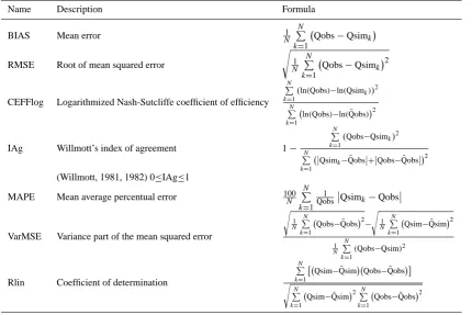
Table 1. Statistical goodness-of-fit measures calculated for the model output (Qobs: observed discharge, Qsim: simulated discharge).

Name Description Formula

BIAS Mean error _N1

N

P

k=1

Qobs−Qsimk

RMSE Root of mean squared error

s 1

N N

P

k=1

Qobs−Qsimk

2

CEFFlog Logarithmized Nash-Sutcliffe coefficient of efficiency

N

P

k=1

(ln(Qobs)−ln(Qsim_k))2

N

P

k=1

ln(Qobs)−ln(Qobs¯ )2

IAg Willmott’s index of agreement 1−

N

P

k=1

(Qobs−Qsim_k)2

N

P

k=1

Qsimk− ¯Qobs

+

Qobs− ¯Qobs 2

(Willmott, 1981, 1982) 0≤IAg≤1

MAPE Mean average percentual error 100_N

N

P

k=1 1 Qobs

Qsim_k−Qobs

VarMSE Variance part of the mean squared error

s

1

N N

P

k=1

Qobs− ¯Qobs2 − s 1 N N P

k=1

Qsim− ¯Qsim2

1

N N

P

k=1

(Qobs−Qsim)2

Rlin Coefficient of determination

N

P

k=1

Qsim− ¯Qsim

Qobs− ¯Qobs s

N

P

k=1

Qsim− ¯Qsim2PN

k=1

Qobs− ¯Qobs2

vectoryonto the discrete output space that has not been part of the training data manifold. This means that according to Eq. (4) a neuronc(y)with reference vectormc(y)is activated for which

y−mc(y)

=min

i

{ky−mik} (7)

The “image”c(y)of the projected data itemythen represents the domain of input data patterns fromXthat is most similar toy. Moreover, as the number of neuronskis much smaller than the number of vectors used for the training, this neuron will be ‘sensitized’ and associated to a number of input data patterns from X which will represent the domain of input data patterns that is closest toy.

2.2 Experimental setup

In our example 4000 residual time series (i.e. the element-wise difference between the simulated and the observed time series vectors) constituted the input data vectors of the train-ing data set. The model time series were obtained from 4000 Monte Carlo simulations (see Sect. 2.3) with the distributed conceptual watershed model NASIM running at hourly time steps over a period of two years, i.e. each input data vec-tor consisted of 17 472 elements. Before the training, nor-malization of the data after Eq. (8) was carried out to avoid that high data values (vector elements) dominate the train-ing because of their higher impact on the Euclidean distance

measure Eq. (3) (Vesanto et al., 2000). Each element of the input data vectors is normalized to a variance of one and zero mean value using the linear transformation

x0=(x− ¯x) /σx. (8)

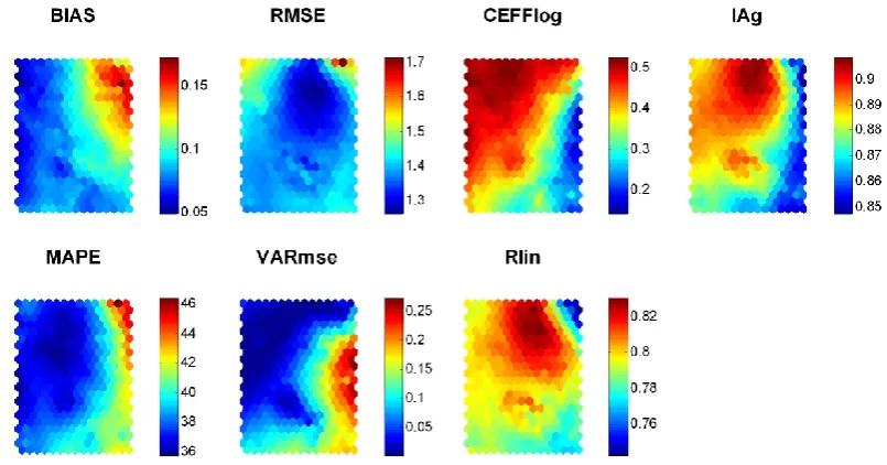
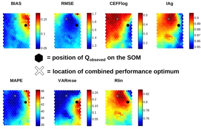
Fig. 2. Distribution of the mean values of each performance measure from Table 2 over the SOM lattice.

optima on the map, each optimum is considered as a mass point with unit weight on the SOM grid. The common opti-mum is calculated as geometric center of mass resulting from the locations of the seven objective function optima. The x-coordinatexoptof the common optimum fornoptima is

cal-culated using Eq. (9)

xopt= P

wixi

P_w

i

, i=1. . .n (9)

wherexiare the x-coordinates of the individual optima on the SOM grid. Heren=7 andwi = 1 for all i. The y-coordinate

yoptis determined accordingly. To ascertain whether the type

of data used for the training exerts any influence on the SOM result the experiments were repeated with a SOM trained on discharge time series instead of residual time series. The SCE-UA algorithm (Duan et al., 1993) for the model opti-mization was run with a maximum of 10 000 iterations and 5 complexes (with 5 points each). For successful termination a change of less than 0.05% of the performance criterion in three consecutive loops was imposed.

2.3 NASIM model and data

NASIM is a distributed conceptual rainfall-runoff model (Hydrotec, 2005). It uses non-linear storage elements to simulate the soil water balance on spatially homogeneous units with respect to soil and land use, which themselves are subdivided into soil layers. NASIM is being commer-cially distributed since the mid-eighties and since then has found widespread application, e.g. in communal water re-sources management throughout Germany. The details of the model are beyond the scope of this contribution. Instead, we adopt the decision-maker’s point of view and treat the model

Table 2. Free NASIM model parameters of the Monte-Carlo

simu-lation with their respective parameter ranges.

Name Description Range

RetBasis Storage coefficient for 0.5–3.5

baseflow component [h]

RetInf Storage coefficient for 2.0–6.0

interflow component [h]

RetOf Storage coefficient for surface runoff 2.0–6.0

from unsealed surfaces [h]

StFFRet Storage coefficient for 2.0–6.0

surface runoff from urban areas [h]

hL Horizontal hydraulic conductivity factor 2.0–8.0

maxInf Maximum infiltration factor 0.025–1.025

vL Vertical hydraulic conductivity factor 0.005–0.105

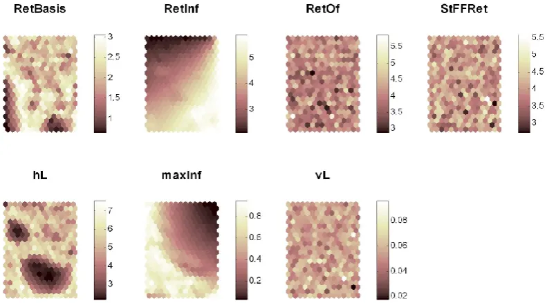
Fig. 3. Distribution of the mean values of each model parameter from Table 1 over the SOM lattice.

3 Results

In the first part of this section the properties of the SOM trained on residual time series and the relation of its elements to the traditional performance measures are examined. The second part is dedicated to testing the projection of measured data onto the SOM.

3.1 Testing the properties of the SOM

After the training each neuron of the 22×15 SOM is expected to be activated by a narrow domain of residual patterns from the input data manifold. The neurons and their respective lo-cation on the map are identifiable by index numbers. As the number of neurons is still much smaller than the number of model realizations used for the training, each neuron repre-sents a set of Monte-Carlo model realizations that are char-acterized through similar temporal patterns with respect to their residuals or discharge values respectively. Because of the topographic ordering principle neighbouring map units, in turn, are expected to be “tuned” to similar residual pat-terns as well. Because the model realizations used for the training can be referenced by their corresponding index num-ber on the map, the ordering principles of the “semantic map” represented by the SOM can be examined. To this end, the means of different performance measures as well as the mean values of the model parameters on each map element are calculated according to Sect. 2.2. This allows to assess the properties of the map’s ordering principle with respect to well known attributes such as (a) the distribution of perfor-mance measures and (b) the distribution of different model parameter values over the map lattice. Referring to (a) seven performance measures have been calculated for each model

realization (Table 1). For each of them individual SOM lat-tices were colour-coded according to the mean of the perfor-mance measure of the model runs associated with each map unit. Figure 2 shows the distribution of the performance mea-sures from Table 1 on the SOM lattice. The same procedure was repeated for the values of the free parameters such that the distribution of mean parameter values can be shown for each parameter individually (Fig. 3). In each lattice of Figs. 2 and 3 the positions of the neurons remain identical such that each map element refers to identical model realizations in both figures.

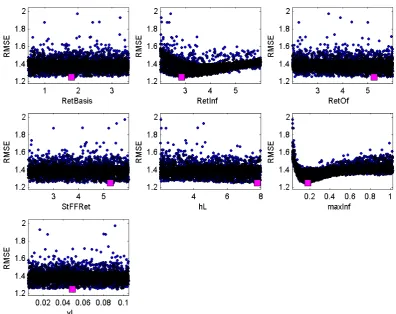
Fig. 4. Scatterplots of RMSE values for each of the examined NASIM parameters.

Table 3. Summary of the parameter values of the 11 model

real-izations associated to the Best-Matching map Unit when the time series vector of observed discharges is projected onto the SOM.

RetBasis RetInf RetOf StFFRet hL maxInf vL

min 0.699 4.336 2.379 2.202 2.191 0.107 0.008

max 3.143 4.787 5.731 5.581 6.540 0.134 0.105

mean 1.756 4.555 4.278 3.548 4.674 0.122 0.065

RetInf and maxInf are sensitive with reference to the RMSE. Scatterplots for the remaining objective functions in Table 1 yielded comparable results. From the aforementioned find-ings we infer that the locally ordered parameter mean values in Fig. 3 (RetBasis and hL) indicate that the corresponding parameters are subject to interaction with other parameters. Results identical to Figs. 2 and 3 were obtained by training a SOM on discharge time series instead of residual values. 3.2 Projecting the observed time series onto the SOM To locate the best-matching unit (BMU) of the measured discharge (i.e. zero-residual) time series on the map, ac-cording to Sect. 2.1, an input vector consisting of elements with value 0 is constructed. Subsequently, in order to be

Table 4. Comparison of model performances for results obtained

from manual calibration, optimization with SCE-UA and the SOM application. In case of the SOM mean values of 11 results are given.

BIAS RMSE CEFFlog IAg MAPE VARmse Rlin

manual 0.32 1.58 0.50 0.86 42.36 0.01 0.75

calibration

SCE-UA 0.10 1.25 0.49 0.91 36.37 0.06 0.83

optimization

SOM 0.13 1.34 0.30 0.88 40.71 0.19 0.81

(means)

BIAS

0.05 0.1 0.15

RMSE

1.3 1.4 1.5 1.6 1.7

CEFFlog

0.2 0.3 0.4 0.5

IAg

0.85 0.86 0.87 0.88 0.89 0.9

MAPE

36 38 40 42 44 46

VARmse

0.05 0.1 0.15 0.2 0.25

Rlin

0.76 0.78 0.8 0.82

= position of Q

on the SOM

= location of combined performance optimum

Fig. 5. The location of the best-matching unit (indicated by the black dot) for an input vector that represents the measured discharge time

series.The white cross marks the common optimum (balance point) of the seven performance measures on the SOM grid.

BIAS

CEFFlog IAg

MAPE

VARmse _{RMSE +} Rlin

’Center of mass’ combined optimum

Fig. 6. Determination of the common optimum location (balance

point) as the geometric center of mass resulting from the locations of the seven obejective function optima on the SOM. Each optimum has unit weight. Here the RMSE and Rlin optima coincide on the same position.

Table 3 summarizes the parameter values of the 11 model re-alizations that are associated to the BMU for representing the model time series that are most “similar” to a “perfect match” (i.e. the zero-residual case). By comparing these parameters

0 5 10 15 20 25

Q [m

³/

s

]

Manual calibration

envelope of all simulations observed discharge manual calibration

0 5 10 15 20 25

Q [m

³/s

]

SCE-UA optimization

envelope of all simulations observed discharge SCE-UA optimization of RMSE

14/01/950 18/02/95 25/03/95 29/04/95 03/06/95 08/07/95 12/08/95 16/09/95 21/10/95

5 10 15 20 25

SOM

Q [m

³/

s

]

envelope of all simulations observed discharge SOM results

(a)

(b)

(c)

max. 38.2

max. 47.3

max. 38.2

max. 47.3

max. 38.2

max. 47.3

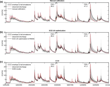
Fig. 7. The model realizations as resulting from (a) manual calibration, (b) optimization with the SCE-UA algorithm and (c) the BMU of the

SOM for the measured discharge time series. The time-series are compared to the measured discharge and the envelope of the Monte-Carlo simulation, i.e. the area which is spanned by all model time series for the bounds given in Table 2.

(Fig. 7b) outperforms the BMU realizations as well as the manual calibration. The RMSE of the SCE-optimized model equals the lowest RMSE value obtainable from the given set of Monte-Carlo realizations. The corresponding hydrograph provides a reasonable representation of the measured time se-ries, except for some deficits in the reproduction of the peak discharges. The SCE-optimized model and the realizations from the BMU display noticeable differences in the repro-duction of the peak discharges and recession limbs. Though, the SCE result, based on a visual examination, slightly out-performs the SOM method. The training on discharge data time series yields identical results with respect to the position of the BMU on the SOM as well as the model realizations that were associated to it.

4 Discussion and conclusions

The performance measures that are linked to the map in Fig. 2 already indicate that very individual properties of the training data time series can be attributed to each element of the Self-Organizing Map. Furthermore, from the patterns of the performance measures on Fig. 2 it can be seen that certain correlation structures inherent to these statistical measures

appear to be reflected by the map. Henceforth, we deduce that the information that can be extracted by these aggregat-ing statistical measures is assimilated and preserved by the SOM. The findings with respect to Fig. 3, corroborated by Fig. 4 and Table 3, demonstrate that the SOM application is capable of revealing information about parameter sensi-tivities and, to a certain degree, parameter interactions. We consider these results an indication of the high discrimina-tive power of the SOM application with respect to the char-acteristics of different simulated discharge time series. This is because we were not able to obtain similar findings with traditional methods that are based on the evaluation of per-formance measures, e.g. parameter response surfaces for dif-ferent objective functions.

objective function values for these time series also suggest a higher accuracy of the results obtained by application of the SCE algorithm. In contrast to the SCE algorithm the resolution of the SOM method is dependent upon the num-ber of model time series that participated in its training. It should be borne in mind that, compared to the number of model parameters, the results given in Fig. 7c are still based on a rather small number of model data items for the SOM training. The results could therefore improve when a more densely sampled dataset is used for the training. Neverthe-less the model realizations that have been attributed to the BMU already exhibit qualities similar to the result which was based on optimization with the SCE algorithm. The differ-ences between these realizations might further be attributed to the fact that the SOM training does not tend to put em-phasis on particular hydrograph features, which however can be expected when using RMSE as optimization criterion. A strong point of the SOM procedure is its ability to provide a number of alternative model realizations that approximate the measured time series equally well. This allows for con-fining the parameter space to a region that closely represents a measured data set and renders the SOM potentially useful for future model identification applications. Most notably it has to be pointed out that the SOM method does not depend on aggregating statistical measures. Consequently the “simi-larity” represented in the SOM is not directly quantifiable in traditional terms. Instead, it rather accounts for the complex-ity that is inherent to time series data and which cannot be reduced to a rank number. Although the method is determin-istic and the results are entirely reproducible, the resulting time series (Fig. 7c) can be further judged only subjectively. The fact that the experiments yielded identical results when the training was carried out using discharge data underpins the stability of the SOM method.

The discriminatory power of the SOM that has been demonstrated in this article also highlights that uncertainty induced by the properties of the performance measure should be included in the discussion of model uncertainties and equifinality, because any statement on model behaviour de-pends on our possibilities to differentiate between model time series.

Acknowledgements. The authors wish to thank O. Buchholz (Hydrotec GmbH) and R. Wengel for their support. This work was carried out using the SOM-Toolbox for Matlab by the

“SOM Toolbox Team”, Helsinki University of Technology

(http://www.cis.hut.fi/projects/somtoolbox).

Edited by: F. Laio

References

Alhoniemi, E., Hollm´en, J., Simula, O., and Vesanto, J.: Process Monitoring and Modeling using the Self-Organizing Map, Integr. Comput.-Aid. E., 6, 3–14, 1999.

Allinson, N. M. and Yin, H.: Self-Organising Maps for Pattern Recognition, in: Kohonen Maps, edited by: Oja, E. and Kaski, S., Elsevier, Amsterdam, 111–120, 1999.

Ambroise, B., Perrin, J. L., and Reutenauer, D.: Multicriterion val-idation of a semidistributed conceptual model of the water cycle in the Fecht Catchment (Vosges Massif, France), Water Resour. Res., 31, 1467–1482, 1995.

Beven, K. J. and Binley, A.: The future of distributed models: model calibration and uncertainty prediction, Hydrol. Process., 6, 279-298, 1992.

Boyle, D. P., Gupta, H. V., and Sorooshian, S.: Toward improved calibration of hydrologic models: Combining the strengths of manual and automatic methods, Water Resour. Res., 36, 3663-3674, 2000.

Cho, J.: Multiple Modelling and Control of Nonlinear Systems with Self-Organizing Maps, PhD Thesis, University of Florida, 130 pp., 2004.

Clemen, T.: Zur Wavelet-gest¨utzten Validierung von Simulations-modellen in der ¨Okologie, Dissertation, Institut f¨ur Informatik und Praktische Mathematik, Christian-Albrechts-Universit¨at, Kiel, 111 pp., 1999.

Duan, Q., Gupta, V. K., and Sorooshian, S.: Shuffled complex evo-lution approach for effective and efficient global minimization, J. Optimiz. Theory App., 76, 501–521, 1993.

Franks, S. W., Gineste, P., Beven, K. J., and Merot, P.: On constrain-ing the predictions of a distributed model: the incorporation of fuzzy estimates of saturated areas into the calibration process, Water Resour. Res., 34, 787–797, 1998.

Gupta, H. V., Sorooshian, S., and Yapo, P. O.: Toward improved calibration of hydrologic models: Multiple and noncommensu-rable measures of information, Water Resour. Res., 34, 751–764, 1998.

Gupta, H. V., Sorooshian, S., Hogue, T. S., and Boyle, D. P.: Ad-vances in Automatic Calibration of Watershed Models, in: Cali-bration of Watershed Models, edited by: Duan, Q., Gupta, H. V., Sorooshian, S., Rousseau, A. N., and Turcotte, R., Water Science and Application, AGU, Washington D.C., 9–28, 2003.

Haykin, S.: Neural networks – a comprehensive foundation, 2nd ed., New Jersey, 842 pp., 1999.

Hsu, K.-l., Gupta, H. V., Gao, X., Sorooshian, S., and Imam, B.: Self-organizing linear output map (SOLO): An artificial neural network suitable for hydrologic modeling and analysis, Water Resour. Res., 38, 1302, doi:10.1029/2001WR000795, 2002. Hydrotec: Rainfall-Runoff-Model NASIM – program

documenta-tion (in German), Hydrotec Ltd., Aachen, 579 pp., 2005. Kalteh, A. M. and Berndtsson, R.: Interpolating monthly

precipi-tation by self-organizing map (SOM) and multilayer perceptron (MLP), Hydrolog. Sci. J., 52, 305–317, 2007.

Kohonen, T.: Self-Organizing Maps, 3rd ed., Information Sciences, Berlin, Heidelberg, New York, 501 pp., 2001.

wavelet analysis, Hydrol. Process., 21, 586–607, 2007.

Legates, D. R. and McCabe Jr., G. J.: Evaluating the use of “goodness-of-fit” measures in hydrologic and hydroclimatic model validation, Water Resour. Res., 35, 233–241, 1999. Lischeid, G.: A decision support system for mountain basin

man-agement using sparse data, EGU General Assembly 2006, Vi-enna, Geophys. Res. Abstr., 8, EGU06-A-04223, 2006. Montanari, A. and Toth, E.: Calibration of hydrological models in

the spectral domain: An opportunity for scarcely gauged basins?, Water Resour. Res., 43, W05434, doi:10.1029/2006WR005184, 2007.

Peeters, L., Bac¸˜ao, F., Lobo, V., and Dassargues, A.: Exploratory data analysis and clustering of multivariate spatial hydrogeolog-ical data by means of GEO3DSOM, a variant of Kohonen’s Self-Organizing Map, Hydrol. Earth Syst. Sci., 11, 1309–1321, 2007, http://www.hydrol-earth-syst-sci.net/11/1309/2007/.

Principe, J. C., Wang, L., and Motter, M. A.: Local dynamic model-ing with self-organizmodel-ing maps and applications to nonlinear sys-tem identification and control, P. IEEE, 86, 2240–2258, 1998. Sch¨utze, N., Schmitz, G. H., and Petersohn, U.: Self-organizing

maps with multiple input-output option for modeling the Richards equation and its inverse solution, Water Resour. Res., 41, W03022, doi:10.1029/2004WR003630, 2005.

Seibert, J.: Multi-criteria calibration of a conceptual runoff model using a genetic algorithm, Hydrol. Earth Syst. Sci., 4, 215–224, 2000,

http://www.hydrol-earth-syst-sci.net/4/215/2000/.

and Modeling of Complex Systems Using the Self-Organizing Map, in: Neuro-Fuzzy Techniques for Intelligent Information Systems, edited by: Kasabov, N., and Kozma, R., Physica Verlag (Springer Verlag), 3–22, 1999.

Vesanto, J.: Using the SOM and Local Models in Time-Series Pre-diction, Workshop on Self-Organizing Maps (WSOM’97), Es-poo, Finland, 1997, 209–214, 1997.

Vesanto, J., Himberg, J., Alhoniemi, E., and Parhankangas, J.: SOM Toolbox for Matlab 5, Helsinki University of Technology, Espoo, 60 pp., 2000.

Vrugt, J. A., Gupta, H. V., Bastidas, L. A., Bouten, W., and Sorooshian, S.: Effective and efficient algorithm for multiob-jective optimization of hydrologic models, Water Resour. Res., 39(4), 1214, doi:10.1029/2002WR001746, 2003.

Wagener, T., Wheater, H. S., and Gupta, H. V.: Identification and Evaluation of Watershed Models, in: Calibration of Watershed Models, edited by: Duan, Q., Gupta, H. V., Sorooshian, S., Rousseau, A. N., and Turcotte, R., Water Science and Applica-tion, AGU, Washington D.C., 29–47, 2003.

Wagener, T., Wheater, H. S., and Gupta, H. V.: Rainfall-Runoff Modelling in Gauged and Ungauged Basins, Imperial College Press, London, 306 pp., 2004.

Willmott, C. J.: On the validation of models, Phys. Geogr., 2, 184– 194, 1981.

Willmott, C. J.: Some Comments on the Evaluation of Model Per-formance, B. Am. Meteorol. Soc., 63, 1309–1313, 1982. Yapo, P. O., Gupta, H. V., and Sorooshian, S.: Multi-objective