www.hydrol-earth-syst-sci.net/13/395/2009/ © Author(s) 2009. This work is distributed under the Creative Commons Attribution 3.0 License.
Earth System
Sciences
Mapping model behaviour using Self-Organizing Maps
M. Herbst1, H. V. Gupta2, and M. C. Casper1
1Department of Physical Geography, University of Trier, Germany
2Department of Hydrology & Water Resources, University of Arizona, Tucson, USA
Received: 25 September 2008 – Published in Hydrol. Earth Syst. Sci. Discuss.: 4 December 2008 Revised: 9 March 2009 – Accepted: 9 March 2009 – Published: 18 March 2009
Abstract. Hydrological model evaluation and identification essentially involves extracting and processing information from model time series. However, the type of information extracted by statistical measures has only very limited mean-ing because it does not relate to the hydrological context of the data. To overcome this inadequacy we exploit the di-agnostic evaluation concept of Signature Indices, in which model performance is measured using theoretically relevant characteristics of system behaviour. In our study, a Self-Organizing Map (SOM) is used to process the Signatures ex-tracted from Monte-Carlo simulations generated by the dis-tributed conceptual watershed model NASIM. The SOM cre-ates a hydrologically interpretable mapping of overall model behaviour, which immediately reveals deficits and trade-offs in the ability of the model to represent the different functional behaviours of the watershed. Further, it facilitates interpre-tation of the hydrological functions of the model parameters and provides preliminary information regarding their sensi-tivities. Most notably, we use this mapping to identify the set of model realizations (among the Monte-Carlo data) that most closely approximate the observed discharge time se-ries in terms of the hydrologically relevant characteristics, and to confine the parameter space accordingly. Our results suggest that Signature Index based SOMs could potentially serve as tools for decision makers inasmuch as model real-izations with specific Signature properties can be selected according to the purpose of the model application. More-over, given that the approach helps to represent and analyze multi-dimensional distributions, it could be used to form the basis of an optimization framework that uses SOMs to char-acterize the model performance response surface. As such it provides a powerful and useful way to conduct model identi-fication and model uncertainty analyses.
Correspondence to: M. Herbst ([email protected])
1 Introduction
Diagnostic model evaluation and identification aim at elu-cidating the extent to which the model is able to represent the observed system behaviour and identifying the reasons why its response is inconsistent with the observations (Gupta et al., 2008). This task – a fundamental step in the iterative model building and identification process – requires adequate tools that guide the modeller towards isolating the causes of “unsatisfactory” model behaviour such that changes to the parameters or the model structure can be made accordingly (Wagener et al., 2003b; Gupta et al., 2008). Model evaluation is commonly based on the comparison of model generated input-state-output simulations with observed historical data. In its simplest, but most powerful, form this is done visually in the course of manual calibration, because a trained expert is able to simultaneously discern various characteristics of the data and relate them to the hydrological context.
of the underlying model hypothesis. Hence, the inability of a model to reproduce the whole time series with a sin-gle parameter set can be indicative of structural model errors (Gupta et al., 1998; Wagener et al., 2003b; Lin and Beck, 2007). However, errors in the forcing data as well as in the parameterization are also frequent causes of temporal param-eter variability.
Even so, evaluation methods that rely on a quantification of the “difference” between the simulation and the measure-ments commonly resort to regression based statistical mea-sures of fit as the primary method of information extraction (Legates an McCabe Jr., 1999; Willmott et al., 1981; Nash and Sutcliffe, 1970). The pitfalls of using such measures are well known (e.g. see Hall, 2001; Lane, 2007; Schaefli and Gupta, 2007). However, when dealing with model evalua-tion in a diagnostic sense, the nature of the ‘informaevalua-tion’ we extract from the input-output data by means of these mea-sures deserves critical attention. Gupta et al. (2008) point out that different types of information can be extracted depend-ing on the context in which the data is placed. By puttdepend-ing data in the context of common statistical measures of fit, we allow primarily for a correlative evaluation of the data; e.g., the correlation coefficient informs about the percentage of the observed variance that can be explained by the model simulation, but conveys little or no information that relates directly to the hydrological context of model/data, e.g. a bias in the water balance, or in the velocity of the rainfall-runoff response.
Because variance-based statistical measures fail to extract and relate the information contained in the model time series data to characteristics that are interpretable and meaningful in the context of the hydrological theory, they offer only min-imal diagnostic support when used at the front end of various model evaluation frameworks. In response to this, Gupta et al. (2008) and Yilmaz et al. (2008) recently proposed the con-cept of a diagnostic evaluation approach rooted in informa-tion theory, in which a set of measures is used to characterize various theoretically relevant system functions and process behaviours. The term “Signature Indices” is introduced to distinguish these measures from conventional variance based performance measures that lack relationships to the underly-ing hydrological theory. Yilmaz et al. (2008) propose a set of such Signature Indices to help guide the diagnostic process of model evaluation in a meaningful and interpretable way, inasmuch as these measures correspond to four major hy-drological functions of the watershed: overall water balance, vertical redistribution, temporal redistribution and spatial re-distribution.
In complementary work, Herbst and Casper (2008) pro-pose a model evaluation approach that circumvents the low discriminatory power of statistical performance measures (Gupta et al., 2003), while maximally exploiting the po-tential information in the data, by use of the power of Organizing Maps (SOMs) (Kohonen, 2001). A Self-Organizing Map consists of an unsupervised learning
neu-ral network algorithm that performs a non-linear mapping of the dominant structures present in a high-dimensional data field onto a lower-dimensional grid. The SOM has found di-verse applications in fields such as pattern recognition, image analysis (Kohonen, 2001), exploratory data analysis (Kaski, 1997; Vesanto, 2000a) in geo-spatial (Lourenc¸o, 2005) as well as hydrochemical data (Boogaard et al., 1998; Lis-cheid, 2006; Peeters et al., 2007), process monitoring (Al-honiemi et al., 1999; Simula et al., 1999), local time se-ries modelling (Vesanto, 1997) and time sese-ries forecasting (Simon et al., 2005). Applications related to hydrological modelling remain far less numerous, albeit rather diverse: Kalteh and Berndtsson (2007) use SOMs for the interpola-tion of monthly precipitainterpola-tion; Lin and Chen (2006) apply SOMs for regional precipitation frequency analysis; Sch¨utze et al. (2005) use an extension of the SOM to approximate the Richards equation and its inverse; Huang et al. (2003), and similarly Rajanayaka et al. (2003), apply SOMs to clus-ter and categorize soil data sets in a framework for estimat-ing model parameters in data-sparse areas; Chang (2001) ex-plores the use of SOMs to infer physical and hydraulic soil properties based on remotely sensed brightness temperature data; Mele and Crowley (2008) apply an SOM to examine the interrelationship between different bio-indicators and hy-drological soil properties.
In the context of watershed modelling, Hsu et al. (2002) successfully performed daily streamflow predictions using an SOM to identify different rainfall-runoff stages to which lo-cal regression functions are assigned – a similar approach is used by Abramowitz et al. (2006) to characterize the system-atic component of land surface model output error in a flux correction technique for land surface models (Abramowitz et al., 2007). Abramowitz and Gupta (2008) also use an SOM to evaluate multi-model independence. A further applica-tion to land surface modelling is presented by Abramowitz et al. (2008) who use SOM to cluster time steps with similar meteorological condition in order to examine the conditional bias of land surface models. Reusser et al. (2008) present another interesting approach in the field of model evaluation. They analyze the temporal dynamics as well as the type of model error by using SOM for the assessment of multiple performance measures from a moving window approach.
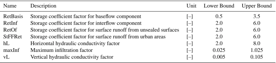
Table 1. NASIM model parameters of the Monte-Carlo simulation with their respective parameter bounds.
Name Description Unit Lower Bound Upper Bound
RetBasis Storage coefficient factor for baseflow component [–] 0.5 3.5
RetInf Storage coefficient factor for interflow component [–] 2.0 6.0
RetOf Storage coefficient factor for surface runoff from unsealed surfaces [–] 2.0 6.0
StFFRet Storage coefficient factor for surface runoff from urban areas [–] 2.0 6.0
hL Horizontal hydraulic conductivity factor [–] 2.0 8.0
maxInf Maximum infiltration factor [–] 0.025 1.025
vL Vertical hydraulic conductivity factor [–] 0.005 0.105
statistical goodness-of-fit measures – because the clustering into SOM nodes is not based on patterns/properties that have direct hydrological relevance, the map is not easy to interpret. Further, because the SOM training involves use of entire (po-tentially very long and/or high-dimensional) time series the computational costs are rather high.
The main goal of this paper is to explore how the Herbst and Casper (2008) SOM-based approach can be improved by linking it to the Signature Index concept (Gupta et al., 2008), which defines the similarity between data items in a more meaningful (hydrologically relevant) way. So, in-stead of working directly with the data time series, the SOM training is conducted on the set of Signature Indices intro-duced by Yilmaz et al. (2008), computed from each of the Monte-Carlo simulation time-series generated by the dis-tributed conceptual hydrological model. In this context, it is interesting to note that the SOM based method presented in this paper in many aspects aims at similar objectives as the Parameter Identification Method based on the Localiza-tion of InformaLocaliza-tion (PIMLI) developed by Vrugt et al. (2001, 2002). The PIMLI method attempts to find disjunctive sub-sets of the observations that contain the most information for the different model parameters. It thus provides a diag-nostic instrument that helps differentiating between param-eters and model concepts. In contrast to the SOM based method PIMLI is a sequential optimization methodology that approaches the model evaluation problem more from the ob-servations than the model itself.
The manuscript is organized as follows; following a brief overview of the model and the data used (Sect. 2.1), we dis-cuss how the hydrologically relevant Signature Indices are computed from model output time series (Sect. 2.2). Sec-tion 2.3 presents a brief discussion of the concept and prop-erties of the Self-Organizing Map, followed by a discussion of the training process (Sect. 2.4). The results are presented in Sect. 3 followed by a discussion (Sect. 4) of possible rea-sons for the differences between the findings presented in this contribution and the results previously published by Herbst and Casper (2008). We conclude with suggestions for other possible applications, and try to illuminate the method in the context of existing model evaluation and optimization meth-ods.
2 Methods
2.1 Model and data
This work employs the same model and data used by Herbst and Casper (2008). Monte-Carlo simulations of hourly stream flow, over a period of approximately two years, were generated using the distributed conceptual watershed model NASIM; see Hydrotec (2005) for details. The model uses a spatial discretization based on sub-catchments. For the “Schwarze Pockau” watershed preprocessing of spatial data resulted in 71 sub-catchments with a mean size of approxi-mately 1.8 km2. These are further subdivided into spatially homogeneous units with respect to soil and land use. Each of these elementary spatial units is again vertically divided into soil layers. All lateral flow components that result from the processes within the elementary units are aggregated on the sub-catchment scale. The NASIM parameters examined in this study (Table 1) are unit less factors that modify in-ternal parameter values that are either based on global de-fault values or have been determined individually for each sub-basin in the course of the spatial data preprocessing: The internal values modified by RetOf are determined in the course of the preprocessing depending on the slope in each sub-basin, while the internal RetInf, RetBas, StFFRet are set to global values. The internal values of maxInf as well as vL are determined according to soil type. The model has been distributed commercially since the mid-eighties, and has found widespread application in water resources man-agement throughout Germany.
In this work, we adopt the decision-maker’s point of view, treat the model as a black-box, and try to understand its functioning via the methods presented in this paper. The test watershed is the low-mountain range 129 km2catchment “Schwarze Pockau” Saxony (Germany), a tributary of the Freiberger Mulde (Elbe sub-basin) situated near the border to Czech Republic.
were generated by randomly varying seven of the model pa-rameters (Table 1), all related to the soil water balance and vertical redistribution of flow components, over their feasible ranges. Because appropriate prior information on parameter (or rather factor) distributions was missing uniform distri-butions were assumed. The variation of these factors dur-ing the Monte-Carlo simulation was performed with global values for all sub-catchments. The ranges for the free pa-rameter factors and the values for the fixed papa-rameter factors were set based on prior knowledge acquired via manual ex-pert calibration to the test watershed. We assume that these values represent the plausible parameter space for this water-shed with very high probability.
2.2 Signature indices
The Signature Indices used in this work were designed with a view to providing generally applicable and meaningful mea-sures of model performance that can provide information helpful in detecting and isolating causes of model inadequa-cies, thereby providing guidance towards model improve-ments (Yilmaz et al., 2008). Unlike standard statistical mea-sures of fit these Signature Indices are rooted in the context of the hydrological theory underlying our conceptual repre-sentation of the watershed. The reason for multiple indices is that each is designed to target different (complementary) aspects of model/system behavior (see Gupta et al., 2008). Following the concepts and mathematical formulation pre-sented by Yilmaz et al. (2008), we focus on five Signature Indices that provide information about the following intrin-sic watershed characteristics:
– overall water balance
– vertical soil moisture redistribution – behaviour of long-term baseflow
Because none of the model parameters investigated in this paper control the streamflow routing and timing, we do not consider here the fourth intrinsic water shed characteristic – temporal redistribution of flow – but details can be found in Yilmaz et al. (2008).
The first Signature Index focuses on the long-term input-output behaviour of the system (volume balance), and there-fore measures the percent bias in overall runoff (%BiasRR). This index is strongly controlled by the evapotranspiration process and any factors that influence the amount of water available for evapotranspiration. The index should therefore be sensitive to the model components and parameters that control these processes. It is computed as
%BiasRR= P
t
(Qsimt−Qobst)
P
t
Qobst ×100. (1)
where Qsim and Qobs denote the simulated and the observed flow respectively. The next four Signature Indices are derived
from the flow exceedance probability curve (also known as flow duration curve, FDC), to represent watershed charac-teristics that act on short to intermediate time scales. Be-cause the FDC characterizes a watershed’s tendency to pro-duce flows of different magnitudes, it is informative regard-ing the vertical redistribution of water within the soil column. Different sections of the flow duration curve can therefore be associated with the occurrence of fast, intermediate and slow runoff responses. Because construction of the FDC in-volves loss of timing information, these indices should be generally insensitive to output timing errors. For catchments with quick (slow) runoff response we expect the FDC mid-segment slope to be steeper (flatter).
The percent error in the FDC mid-segment slope is given by %BiasFDCm:
%BiasFDCm= (2)
log(Qsimi)−log(Qsimj)
− log(Qobsi)−log(Qobsj)
log(Qobsi)−log(Qobsj)
×100
whereiandj denote the lower and the upper threshold of flow exceedance probability that define the mid-segment of the flow duration curve. The volume of water corresponding to the high flow segment is also useful in a diagnostic con-text; this property is measured as the percent error in FDC high-segment volume %BiasFHV:
%BiasFHV= P
h
(Qsimh−Qobsh)
P
h
(Qobsh) ×100 (3)
wherehdenotes the indices of all discharge values with ex-ceedance probabilities lower than 0.02. Similarly, the vol-ume of water corresponding to long-term base flow is mea-sured as the percent error in the FDC low-segment volume %BiasFLV:
%BiasFLV= (4)
L P l=1
(log(Qsiml)−log(QsimL))− L P l=1
(log(Qobsl)−log(QobsL)) L
P l=1
(log(Qobsl)−log(Qobsl))
×100
%BiasFMM= (5) log(Qsimmedian)−log(Qobsmedian)
log(Qobsmedian) ×100
where Qsimmedian and Qobsmedian denote the median value of the observed and the simulated flow respectively. %Bi-asFMM characterizes differences in the mid-range flow lev-els between simulated and observed discharge. We observed, during this study, that this index is sensitive to errors in the recession limb of the flow hydrograph, specifically in the re-gion of its inflection point.
Note that these indices achieve diagnostic value because a) the functions they measure must be represented in the model to enable proper reproduction of the system behaviour and b) they relate to aspects of the model structure/behavior that act on different time scales. However, we make no claim that this set of indices is comprehensive in representing the various characteristics that describe the behaviour of a water-shed; in this regard, much research on Signature Index design and selection still needs to be done.
Based on the examination of the FDC for the observed discharge, the flow exceedance probability thresholds used in the definition of %BiasFHV, %BiasFDCm and %BiasFLV were subjectively set toi=20% andj=55% respectively. Ac-cordingly, the indexlin Eq. (4) denotes all discharge values with flow exceedance probabilities higher than 55%. Based on Eq. (1)–(5) the characteristics of a simulated time series of discharges can be described in a hydrologically meaningful way by a vector consisting of five Signature Indices. 2.3 The Self-Organizing Map
The Self Organizing Map is an artificial neural network tech-nique designed to help in extracting structure from high-dimensional data sets (e.g. see Kohonen, 2001; Haykin, 1999; Kaski, 1997). Kohonen (2001) provides an exhaus-tive discussion of the algorithm and its properties. An SOM consists of a regular grid G of k neurons; in our case the neurons were arranged on a two-dimensional hexag-onal grid, although other variants are common (Kohonen, 2001). Let X represent a set of Signature Index vectors, x=[x1, x2, . . . , xn]T ∈ <n withn=5, that has been calcu-lated according to Sect. 2.2 for a set of simucalcu-lated discharge time series. Correspondingly, each neuroni=1. . .kofGis represented through a reference vector
mi =[µi1, µi2, . . . , µin]T ∈ <n (6)
whose dimensionnequals the number of elements in an input data vectorx ∈ X. Typically, the reference vectorsmi are initialized to small random values. However, to assure faster and more reliable convergence of the map, we initialize the mi along the two greatest principal component eigenvectors of the data (Kohonen, 2001). The SOM is trained iteratively:
In the first step an input data itemx ∈Xis randomly selected and the Euclidean distance
di =
v u u t
n
X
j=1
xj−mij2 i=1. . . k;j =1. . .n (7)
between x and each reference vector mi is computed (of course, any appropriate metric can be used as a measure of similarity). The “winning neuron” (also called the best-matching unit, BMU, ofx) is the map elementcwhose ref-erence vectormc has the smallest distancedc toxand thus satisfies the condition
dc =min i
{|x−mi|} i=1. . .k. (8)
In the next step the reference vector mc (which corre-sponds to our current best-matching unit) and all reference vectors of its neighbouring neurons are updated according to mi(t+1)=mi(t )+α (t ) hci(t )[x(t )−mi(t )] (9) wheremi(t )is the current weight vector at iteration stept. Thus, the rate of change for each node of the map is scaled by three factors: a) the difference (x(t )−mi(t )) between the input data setx and the prototype vectormi b) the size of a neighbourhood functionhciwhich decreases monotoni-cally to zero withtand with distance from the winning neu-ron and c) a learning rate factorα(t) which gradually lowers the height of the neighbourhood function as the iteration ad-vances. Forhciit is common to use the Gaussian function
hci(t )=exp −
krc−rik2 2σ2(t )
!
(10)
whereσ(t) defines the width of the topological neighbour-hood, and bothσ(t) in Eq. (10) andα(t) in Eq. (9) decrease monotonically witht. Note that an exact choice of the func-tionα(t) is not required (Kohonen, 2001). In this way, the SOM combines elements of competitive and adaptive learn-ing. Repeated cycling through the training steps causes dif-ferent nodes and regions of the map to be “tuned” to spe-cific domains of the input space. Importantly, the enforced local interaction between the SOM nodes, implemented by Eq. (9), results in the map gradually developing an ordered and smooth representation of the input data space (Kaski, 1997).
each training cycle. The reference vectors are updated ac-cording to the weighted average of the data samples
mi(t+1)= N
P
l=1
hci(t )xl
N
P
l=1
hci(t )
(11)
wherecis the index number of the BMU of data setxl, and
Nis the number of data samples. This variant of the training does not make use of the learning rate factorα(t).
The adaptive and competitive learning process of the SOM along with its ability to provide a visualization of the data mapped onto a two-dimensional grid confers properties to the SOM which make it especially interesting for exploratory data analysis (Kaski, 1997). It results in an ordered repre-sentation of complex (i.e. multi-dimensional) data in which items associated with neighbouring nodes of the grid are characterized by similar patterns/properties, which facilitates the perception of structures inherent to the data. Further, patterns that occur more frequently in the input space are mapped onto a larger area. Additionally, the final reference vectors form a discrete approximation of the input data dis-tribution by representing local conditional expected values of the data. They can thus be seen as essentially equivalent to a discretized form of principal curves (Kaski, 1997; Haykin, 1999). Consequently, depending on the scope of its applica-tion, SOM can be used to disclose the clustering structure of the data, or be interpreted as a dimensionality reduction or data compression method.
Finally, the SOM also allows the projection of an input data itemy(in our study a vector of Signature Indices) that has not been part of the training data onto the output space. This means that according to Eq. (8) the neuronc(y) with reference vectormc(y)is determined that satisfies the condi-tion
y−mc(y)
=min
i
{ky−mik}i=1. . .k. (12)
Neuronc(y) then represents the domain of input data pat-terns (i.e. Signature Index patpat-terns) fromXthat is most sim-ilar toy. In turn, the data itemsXc⊂Xwhich are attributed tocare those among the training data items that are most similar toywith respect to the criterion given by Eq. (7) and Eq. (12).
2.4 Data preparation and training
In this work, the training data setX for the SOM was ob-tained by computing the five aforementioned Signature In-dices for each of the 4000 model output time series obtained with NASIM as described in Sect. 2.1 and 2.2. Prior to the training, each Signature Index was normalized to a value hav-ing zero mean and variance of one ushav-ing the linear transfor-mation
x0=(x− ¯x)σx (13)
so that high index values do not exert a disproportionate in-fluence on the training via Eq. (7). The number of neurons, i.e. map units, was determined using the heuristic equation
m=5
√
N whereN=4000 is the total number of data items inX. The side lengths of the map are calculated based on the ratio of the two biggest eigenvalues of the covariance matrix ofX (Vesanto et al., 2000). The training was conducted in two consecutive steps. First, a coarse training period of 500 iterations was performed, using a large radius for the neigh-bourhood function. Subsequently a fine tuning period com-prising 10000 training cycles was performed using a small neighbourhood radius. A hexagonal grid was chosen to help preserve proper topologic relationships. A simple measure of the “quality” of the map is the “quantization error” (Vesanto, 2000a), which represents the average distance of each data vectorxpto its corresponding BMUmc(p), calculated as:
¯
d = 1
N
N
X
p=1
xp−mc(p)
(14)
whereNis the total number of data itemsXused for training, andpis the index of the data items.
According to Eqs. (1)–(5) the Signature Index values as-sociated with the time series of observed discharges Qobs maps asy=[0 0 0 0 0]T into the Signature Index space. Using the transformation Eq. (13) that has been applied to the train-ing data and Eq. (12) the map element c(y) and its related data items Xc were determined that correspond to the Sig-nature Index vector of the time series of observed discharges y=[0 0 0 0 0]T. We will refer toc(y) as the “best-matching unit” (BMU) of the observed data.
As an independent reference point for this result, we used the Shuffled Complex Evolution optimization algorithm (Duan et al., 1992) to find a model realization (parameter set) that minimizes the Root Mean Squared Error (RMSE) of the simulated discharge time series. The SCE-UA algorithm was run with 5 complexes (5 points each) and a maximum of 10 000 iterations. For successful termination a change of less than 0.05 percent of the RMSE in three consecutive loops was imposed.
As a further reference point we conducted a SOM train-ing accordtrain-ing to Herbst and Casper (2008), ustrain-ing the dis-charge time series from the Monte-Carlo simulation as train-ing data. The preprocesstrain-ing was carried out similarly, apply-ing the abovementioned transformation Eq. (13) to each time step of the training data set. For further details regarding this training please see Herbst and Casper (2008).
3 Results
3.1 Properties of the map
Fig. 1. Distribution of reference vector Signature properties. Note
that in each plot the colours are scaled individually.
Fig. 2. Component planes of the SOM rescaled according to the
normalized absolute values of the reference vectors clearly highlight the locations of individual Signature Index optima on the map.
total number of data items used for training. Consequently, every neuron represents a set of simulation runs and their respective Signature Index patterns. As the reference vec-tors of the map are readily accessible, the properties of the individual nodes, with regard to their Signature Index char-acteristics, can be evaluated: The de-normalized reference vectors represent the “prototype patterns” by which the in-dividual neurons are activated. Further, we take advantage of the fact that the input data items attributed to each neuron via the training are referenced. Because each input data item is linked to a parameter set and its resulting simulated time series, the neurons of the map can be evaluated with respect to the model parameters and the properties of the time series.
BMU
Node 53
Node 74
%BiasRR %BiasFDCm %BiasFHV
%BiasFLV %BiasFMM
BMU
BMU
Node 53
Node 53
Node 74
%BiasRR %BiasFDCm %BiasFHV
%BiasFLV %BiasFMM %BiasRR
%BiasFDCm %BiasFHV
%BiasFLV %BiasFMM %BiasRR
%BiasFDCm %BiasFHV
%BiasFLV %BiasFMM
2
3
4
5
6
7
Figure 3. The distribution of Signature Index properties on the map displayed as bar-plots and
the location of the best-matching unit (BMU) on the map. The bars are individually scaled
over the range of each Signature Index such that the topmost position of each bar marks its
absolute maximum and vice versa. Details on properties of the model realizations projected
onto node 53 and 74 are exemplified in Fig. 4.
32
Fig. 3. The distribution of Signature Index properties on the mapdisplayed as bar-plots and the location of the best-matching unit (BMU) on the map. The bars are individually scaled over the range of each Signature Index such that the topmost position of each bar marks its absolute maximum and vice versa. Details on properties of the model realizations projected onto node 53 and 74 are exem-plified in Fig. 4.
[image:7.595.50.291.63.242.2] [image:7.595.49.290.290.485.2]dd/mm/1995
Q [
m
³/
s
]
14/01 11/03 06/05 01/07 26/08 21/100 5
10 15 20 25
Flow exceed. probab. %
Q
[m
³/
s
]
0 50 100
10-1 100 101 102
dd/mm/1995
Q
[m
³/
s
]
14/01 11/03 06/05 01/07 26/08 21/100 5
10 15 20 25
Flow exceed. probab. %
Q [
m
³/
s
]
0 50 100
10-1 100 101 102
envelope of all simulations observed discharge SOM results
%BiasRR %BiasFDCm %BiasFHV
%BiasFLV %BiasFMM
Node 53: Node 74:
d
a
c
[image:8.595.51.284.62.278.2]b
Fig. 4. Examples for Signature Index properties on different
loca-tions of the map (see Fig. 3): Comparison of hydrographs and flow duration curves for the observed discharge and the model realiza-tions projected onto each of the two nodes.
and therefore reveals which capabilities in reproducing the characteristics of the measured time series are mutually ex-clusive. To accentuate the location of individual Signature Index optima on the map Fig. 2 shows the component planes rescaled according to normalized absolute values of the ref-erence vectors. Here, it becomes evident that the model op-tima, with respect to the Signature Indices, are in part mu-tually exclusive. Figure 3 further summarizes the character-istics of the reference vectors: here the Signature Indices of each reference vector are presented as bar-plots where each of the five color-coded bars corresponds to one of the Sig-nature Indices. Note that the bars are individually scaled over the pertinent range of each Signature Index such that the topmost position of each bar marks its absolute maximum and vice versa. From Fig. 3 it can easily be discerned that the model realizations for which all Index values are closest to zero are projected to the neurons located around the left lower third of the map. (The location of the BMU accord-ing to Sect. 2.4 will be determined in the followaccord-ing section). The lower and lower right region of the map is dominated by model realizations with negative Index values regarding %BiasFDC and %BiasFHV which gradually switch over to positive values towards the upper left segment of the map. It is evident from Fig. 1 and 3 that the SOM provides a smooth mapping of the Signature Index properties such that neigh-bouring locations on the map bear similar characteristics with respect to the Signature Indices. The simulations that are rep-resented by the neurons located in the upper left corner of the map (e.g. node 53 in Fig. 3) show positive values of %Bi-asRR, %BiasFDCm and %BiasFHV while at the same time
Fig. 5. Mean values of each model parameter for the simulations
projected onto the individual map elements.
the values of %BiasFLV and %BiasFMM are among the low-est of the training data set. The hydrograph- and exceedance probability plots in Fig. 4a and b confirm that such Signa-ture characteristics are indicative of model realizations with runoff components that react predominantly faster than the measured discharge time series whereas the quick recession of flow translates into volume errors in the intermediate flow components (i.e. higher and narrower flow hydrographs fol-lowing storm events). Additionally, the positive deviation in overall water balance compared to the measured streamflow (i.e.˜high %BiasRR) combined with underestimation of low-flow volume corroborates that, on average, too much volume of flow is allocated to peak discharges. Note that the barplots as well as the component planes (Fig. 1) represent the relative scale of the Signature Indices.
Model realizations projected onto a neuron in the lower left part of the map (e.g. node 74 in Fig. 3), on the other hand, display a very different behaviour, as exemplified in Fig. 4c and d: From the combination of negative asFDCm and %BiasFHV in conjunction with positive %Bi-asFLV and close to zero %BiasRR, it immediately becomes comprehensible that these simulations are marked by overall underestimation of peak flows, delayed recession of flow and overestimation of volume in the low flow component.
[image:8.595.308.546.62.198.2]Fig. 6. Comparison of SOM trained on simulated discharge time
series (a) and the SOM trained on Signature Indices (b) by means of Signature Index mean values for the simulations which are at-tributed to each node. The black dot indicates the position of the BMU of the measured discharge time series. In (c) the SOM based on Signature Indices is represented by the mean values of four sta-tistical performance measures – the root mean square error (RMSE), the Nash-Sutcliffe coefficient of efficiency (CEFF), Willmott’s In-dex of Aggreement (IAg) and the correlation coefficient (Rlin) – that were calculated calculated over the sets of model realizations that are projected onto each neuron.
runoff bias %BiasRR. Likewise, parameter RetInf obviously controls the velocity of the runoff reaction, i.e. the vertical distribution of flow components, and the volumina allocated to high flows as can be observed by the good correspondence with the pattern of %BiasFDCm and %BiasFHV. The pa-rameters RetOf, StFFRet and vL on the other hand display an irregular, “noisy” pattern in the distribution of parame-ter values over the map which does not correspond to any of the patterns present in the Signature Indices. Parameter hL shows the same irregular pattern over wide parts of the map but also presents isolated areas where the parameter values seem to be closely related to the ordered structure of the map (whose structure is governed by Signature Index properties). The aforementioned results lead us to infer that this pattern is likely to be indicative of partial parameter sensitivity, i.e. pa-rameter interaction involving threshold behaviour. The pat-tern displayed by RetOf, StFFRet and vL, on the other hand, can only be explained if changes made to these parameters either did not relate to any of the Signature Indices or if the effect of these parameters were strongly tied to other param-eter values in a highly nonlinear way.
Finally, we compare the ordering principle of the time se-ries map computed by Herbst and Casper (2008) to the cur-rent map based on Signature Indices. For the former case, the mean values of the individual Signature Indices are cal-culated over the sets of time series that are projected onto each neuron of the map. Similar to the component plane vi-sualization in Fig. 1 these mean Signature values are sub-sequently used to colour the map (Fig. 6a). Accordingly, the mean values of the Signature Indices are determined for the neurons of the Signature Index map in order to allow for proper comparability (Fig. 6b). (Note that the de-normalized reference vectors only refer to the properties of the neuron which are acquired during the training, whereas the element-wise mean values of the data items refer to the properties of the data which is projected onto these neurons). In Fig. 6 it is clearly noticeable that the arrangement of the data items on both maps agrees very well with respect to %BiasFDC, %BiasFMM and, to some extent, %BiasFHV. The compo-nents %BiasRR and %BiasFLV show almost identical pat-terns on both maps, which however are inversely arranged in each case.
a
b
c
max. 38.2
max. 47.3
max. 38.2
max. 47.3
max. 38.2
[image:10.595.46.544.63.320.2]max. 47.3
Fig. 7. Comparison of model realizations for the BMU corresponding to the observed discharge time series. (a) The results of the SOM
training on Signature Indices are contrasted to (b) the training on entire time series vectors and (c) the solution obtained by minimizing the RMSE using SCE-UA.
not possible to establish a clear relationship between the Sig-nature Indices and the performance measures. With regard to the position of the optima on both mappings, it can be seen that the BMU in Fig. 6b does not coincide with the optima of the performance measures in Fig. 6c.
3.2 Projection of measured discharge time series onto the map
In Fig. 3 we also mark the location of the BMU of Qobs which was determined according to Sect. 2.4. Figure 3 shows that the BMU identifies a neuron with a reference vector that represents a compromise in minimizing all Signature In-dices. In the following, we will further examine the model-realizations which are attributed to the BMU by virtue of the training process: Fig. 7a shows the 9 hydrographs re-trieved from the BMU of the SOM training on Signature In-dices along with the observed time series and the envelope of the entire Monte-Carlo data set. As can be seen, these hy-drographs comprise rather similar model realizations, com-pared to the total range of Monte-Carlo simulations. In con-trast, Fig. 7b shows the 7 time series obtained from iden-tifying the BMU on a SOM that was trained on the entire time series of the model outputs (as per Herbst and Casper, 2008), without previously converting them to Signature In-dices. Finally, Fig. 7c offers a comparison with the result obtained from minimizing the RMSE using SCE-UA (Duan et al., 1992). The time series that result from the training
on Signature Indices are not as densely bundled within the total range of Monte-Carlo simulations than their counter-parts from Fig. 7b. However, they offer a close approxima-tion to the observed time series, which according to visual examination of the data appears to outperform the SCE-UA algorithm, at least during peak discharges. We further sub-ject these results to a closer examination and also compare the flow duration curves that correspond to the BMU sim-ulations of both training types to the SCE-optimized model and the observed discharges (Fig. 8). Within the range of the available Monte-Carlo output, the model realizations that correspond to the BMU of the SOM trained on Signature In-dices (Fig. 8a) yield a rather close approximation to the flow exceedance probability characteristics of the measured data, with the exception of the low flows. The same holds true for the results obtained from the training on time series. The most notable differences regarding the flow duration curves affect the exceedance probability range between 10 and 20%, where the training on time series leads to better results, and all values below 2% exceedance probability, where the re-alizations obtained from the Signature Index trained SOM perform slightly better.
Fig. 8. Comparison of flow duration curves for simulations
at-tributed to the BMU.
the BMU of the observed data (Qobs) on this map amounts to 1.1. This means that, in terms of the Signature Indices, the average distances between the model simulations and their corresponding BMU are not very much smaller compared to the dissimilarity between the reference vector of the BMU and the observed discharges. Consequently the observed dis-charge time series cannot be exceedingly different from the time series of the training data set and shows good correspon-dence with its BMU.
Comparing the Signature Index ranges of the model re-alizations projected to this BMU to the ranges of the entire Monte-Carlo data set (Fig. 9) the similarity of the simulations on this node, in terms of Signature Indices, as well as the compromise involved with minimizing the Signature Indices by identifying the BMU becomes visible. For all models the range of variation in overall water balance (%BiasRR) ap-pears to be almost negligible when compared to the ranges of the remaining Signature Indices. The Signature Indices
cal-Fig. 9. Comparison of individual Signature Index ranges for the
BMU-realizations corresponding to the SOM training on Signature Indices and the training on time series. Additionally, the Signature Indices obtained from minimizing the RMSE using the SCE-UA algorithm are displayed.
culated for the simulations attributed to the BMU of the SOM trained on time series, on the other hand, also show only moderate variation. Marked differences in the behaviour of these simulations, however, can be stated regarding the per-cent error in the FDC low-segment volume %BiasFLV. Here, the results obtained from the BMU of the SOM based on Signature Indices outperform the corresponding model real-izations from the time series map. The result obtained by minimizing the RMSE using the SCE-UA algorithm displays Signature Index properties that are very similar to both of the aforementioned BMU realizations. Interestingly, the SCE-UA results perform slightly worse with respect to %BiasFHV and markedly better with respect to %BiasFLV, compared to most of the BMU realizations. This finding, however, does not fully coincide with the result suggested by the position of the RMSE optimum relative to the BMU: According to Fig. 6b and c the results for %BiasFLV are generally sup-posed to deteriorate towards the position of the RMSE op-timum which lies approximately three map units above the BMU.
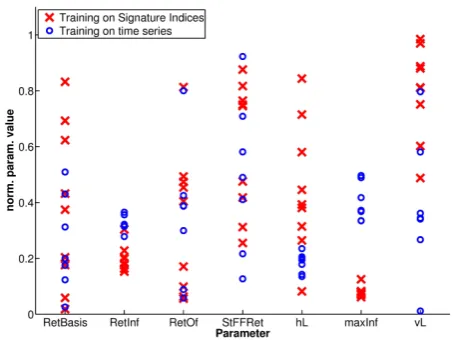
[image:11.595.312.541.63.234.2] [image:11.595.52.285.65.434.2]Fig. 10. Normalized ranges of parameter values retrieved from
the BMUs of the SOM trained on Signature Indices and the SOM trained on time series.
to the location of the BMU, which in case of parameter hL coincides with a map region that lacks an orderly pattern with respect to the parameter values. The corresponding position of the BMU for the training on time series obviously falls into a map region where this is not the case and consequently its range in Fig. 10 is narrowly constrained.
4 Discussion and conclusions
The abovementioned results of our study are the product of two combined approaches: The Signature Measures serve to extract information from model time series data and, at the same time, considerably reduce the amount of data to be dealt with within the SOM algorithm. Gupta et al. (2008) and Yilmaz et al. (2008) argue the hydrological relevance and di-agnostic value of such information for tracking inadequacies in watershed models and for guiding appropriate model im-provements. By using the measures presented in Sect. 2.2, each time series is projected into a five-dimensional Signa-ture Index Space. The underlying assumptions of our study, common to many multi-criteria evaluations, are that the Sig-nature Indices are equally relevant and that the model is ca-pable of reproducing the Signature Index spaces. The role of the Self-Organizing Map, in the second step of our ap-proach, is to produce a discretized (and consequently data-compressed) mapping of the distribution in the Signature In-dex space onto a two-dimensional plane such that the patterns of hydrologically relevant information from a great number of model realizations can be conveyed in a comprehensive manner. In addition, the distribution of hydrologically rel-evant model properties is also linked to the corresponding parameter space that produced the model time series. The difference to the approach by Herbst and Casper (2008) lies in processing the raw time series data into informative indi-cators of hydrological model behaviour. Because in this step
the number of elements in each data item is reduced from several thousand time steps to 5 Signature Indices the di-mensionality and thus the computational burden of training the Self-Organizing Map has been shrunk immensely such that 10 000 training cycles can now be completed in several minutes instead of requiring several days (all computations have been carried out on a 2×Dual-Core Opteron™ Server running at 2.59 GHz).
The high degree of correspondence in Signature patterns on both SOMs shown in Fig. 6 clearly suggests that the Sig-nature Indices have been successfully extracted and have re-produced relevant parts of the information contained in the simulated time series. This, in a sense, points at a high de-gree of equivalence regarding the discriminatory power of the two SOM approaches and underscores the efficiency of using Signature Indices for SOM training on model output data. The comparison of Fig. 6a and b as well as Fig. 9 sug-gests that the SOM trained with time series data and the SOM based on Signature Indices most notably differ with respect to the representation of the long-term behaviour of the sys-tem. From the comparison of Fig. 6b and c it further becomes apparent that an SOM trained on the statistical performance measures used in Fig. 6c most probably would have extracted less independent “information” from the model data.
As some of the Signature Indices are derived from the flow exceedance probability curve it goes without saying that, despite their diagnostic value, not all Signature Indices are completely independent. On the other hand, it has been demonstrated that the way these measures covary for a given set of simulations can reveal much about the behaviour of the model. Most notably, model deficits and trade-offs in representing different watershed functions can immediately be visualized using adequate techniques for reproducing the SOM.
Herbst and Casper (2008) have already shown that prelim-inary information on parameter sensitivities can be provided by training a SOM on model output data. Using the SOM in conjunction with Signature Indices additionally allows us to interpret the function of individual model parameters in the context of hydrological theory even when completely ignor-ing the model structure.
The results from Sect. 3.1 have shown that the ability of a SOM to process and visualize multidimensional data can be exploited successfully for comprehending model behaviour in the hydrological context. Therefore, the SOM approach presented in this contribution also potentially constitutes a valuable tool for decision makers in as much as model re-alizations with specific Signature properties can be selected according to the purpose of the model application (an exam-ple is given in Fig. 4).
[image:12.595.53.281.63.233.2]discharge time series appears to be acceptable compared to the average quantization error of the map. Note that a com-parison between the average quantization errors achieved with the Signature Index SOM and the SOM trained on time series is not very meaningful due to extremely different di-mensionalities of the input data spaces. The results given in Sect. 3.2 indicate that using the Signature Indices has positive effects on the way the SOM can be used to discriminate be-tween different model realizations which consequently bring about improvements regarding the use of the SOM to identify the model results which most closely approximate a given time series. These improvements are probably attributable to the fact that using a set of Signature Indices for the SOM training (theoretically) attributes equal weights to the indi-vidual characteristics considered by them. When training on time series, however, the influence of particular events (e.g. high flow periods) on the SOM training is proportional to their frequency in the data. Thus, although only 4000 model simulations were available, the selection of the “op-timal” models on the basis of a SOM trained on Signature Indices was sufficiently effective (and efficient) that, based on visual examination, the optimization using SCE-UA is outperformed. Of course, as only 4000 model realizations were used, the parameter space was quite sparsely sampled, and adding more data items to the training data set could eas-ily help to refine these results. Because, in a general sense, a SOM can be understood as a means for capturing and analyz-ing multi-dimensional distributions it seems to be well suited for use in model identification and model uncertainty analy-sis. Based on the aforementioned results we suggest that the present SOM approach may constitute an initial step towards an alternative framework for model analysis and optimiza-tion. Further research could therefore, among other topics, be dedicated towards finding efficient re-sampling strategies to explore the parameter space. As to the aspect of using the SOM for multi-criteria optimization, it should be borne in mind that determining the BMU of the measured time series is equivalent to converting a multi-objective optimization to a single-criterion problem by means of weighting the objec-tive function (Zadeh, 1963; Madsen, 2003). This might be of importance in cases where the multi-criteria Pareto front is non-convex; i.e. in general finding the BMU might not pro-vide a genuine multi-criteria solution.
The Signature Indices used here by no means make a claim to completely cover all relevant information contained in the data and a series of other hydrological Signatures are easily imaginable, such as e.g. measures related to the representation of the snow cover or the height and tim-ing of peak discharges. Just as little is known concerntim-ing the requirements of a “parsimonious” description of model behaviour/excluding redundant information on model be-haviour. Therefore, further research on the development of SOM-based applications in the field of hydrological mod-elling will inevitably be confronted with the question of what constitutes a sufficient and informative metric/set of
Signa-ture Measures and the question concerning the number of neurons required to describe the behaviour of a model. This again leads to the more general problems of time series data mining. Defining and identifying the information content of the data constitutes the key towards a more meaningful and precise application of SOM and all other frameworks for the evaluation and analysis of hydrological models.
Acknowledgements. The authors would like to express their
gratitude to Oliver Buchholz (Hydrotec GmbH, Aachen) and Ren´e Wengel. Financial support for this research provided by the German Academic Exchange Service (DAAD, grant D/07/49489) and the German Federal Ministry of Education and Research (BMBF, grant 0330699D) is gratefully acknowledged. We would like to thank the anonymous reviewers and the handling editor for their constructive comments that greatly helped improving this paper.
Edited by: J. Vrugt
References
Abramowitz, G., Gupta, H. V., Pitman, A., Wang, Y., Leun-ing, R., Cleugh, H., and Hsu, K.-l.: Neural Error Regression Diagnosis (NERD): A Tool for Model Bias Identification and Prognostic Data Assimilation, J. Hydrometeorol., 7, 160–177, doi:10.1175/JHM479.1, 2006.
Abramowitz, G., Pitman, A., Gupta, H. V., Kowalczyk, E., and Wang, Y.: Systematic Bias in Land Surface Models, J. Hydrom-eteorol., 8, 989–1001, doi:10.1175/JHM628.1, 2007.
Abramowitz, G. and Gupta, H. V.: Toward a model space and model independence metric, Geophys. Res. Lett., 35, L05705, doi:10.1029/2007GL032834, 2008.
Abramowitz, G., Leuning, R., Clark, M., and Pitman, A.: Evalu-ating the Performance of Land Surface Models, J. Climate, 21, 5468–5481, doi:10.1175/2008JCLI2378.1, 2008.
Alhoniemi, E., Hollm´en, J., Simula, O., and Vesanto, J.: Process Monitoring and Modeling using the Self-Organizing Map, Integr. Comput. Aid. E., 6, 3–14, 1999.
Ambroise, B., Perrin, J. L., and Reutenauer, D.: Multicriterion val-idation of a semidistributed conceptual model of the water cycle in the Fecht Catchment (Vosges Massif, France), Water Resour. Res., 31, 1467–1482, 1995.
Boogaard, H. F. P. v. d., Mynett, A. E., and Ali, M. S.: Self organiz-ing feature maps for the analysis of hydrological and ecological data sets, in: Hydroinformatics ’98, edited by: Babovic, V. M. and Larsen, L. C., Balkema, Rotterdam, The Netherlands, 733– 740, 1998.
Boyle, D. P., Gupta, H. V., and Sorooshian, S.: Toward improved calibration of hydrologic models: Combining the strengths of manual and automatic methods, Water Resour. Res., 36, 3663– 3674, 2000.
Chang, D.-H.: Analysis and modeling of space-time organization of remotely sensed soil moisture, Department of Civil and Environ-mental Engineering, University of Cincinnati, Cincinnati, Ohio, USA, 169 pp., Ph. D. thesis, 2001.
Franks, S. W., Gineste, P., Beven, K. J., and Merot, P.: On constrain-ing the predictions of a distributed model: the incorporation of fuzzy estimates of saturated areas into the calibration process, Water Resour. Res., 34, 787–797, doi:10.1029/97WR03041, 1998.
Gallart, F., Latron, J., Llorens, P., and Beven, K.: Using internal catchment information to reduce the uncertainty of discharge and baseflow predictions, Adv. Water Resour., 30, 808–823, doi:10.1016/j.advwatres.2006.06.005, 2007.
Gupta, H. V., Sorooshian, S., and Yapo, P. O.: Toward improved calibration of hydrologic models: Multiple and noncommensu-rable measures of information, Water Resour. Res., 34, 751–764, 1998.
Gupta, H. V., Sorooshian, S., Hogue, T. S., and Boyle, D. P.: Ad-vances in Automatic Calibration of Watershed Models, in Cali-bration of Watershed Models, edited by Duan, Q., Gupta, H. V., Sorooshian, S., Rousseau, A. N., and Turcotte, R., Water Science and Application Series Vol. 6, AGU, Washington DC, USA, 9– 28, 2003.
Gupta, H. V., Wagener, T., and Liu, Y.: Reconciling theory with observations: elements of a diagnostic approach to model eval-uation, Hydrol. Process., 22, 3802–3813, doi:10.1002/hyp.6989, 2008.
Hall, M. J.: How well does your model fit the data? J. Hydroin-form., 3, 49–55, 2001.
Haykin, S.: Neural networks - a comprehensive foundation, 2nd ed., New Jersey, USA, 842 pp., 1999.
Herbst, M. and Casper, M. C.: Towards model evaluation and iden-tification using Self-Organizing Maps, Hydrol. Earth Syst. Sci., 12, 657–667, 2008,
http://www.hydrol-earth-syst-sci.net/12/657/2008/.
Hsu, K.-L., Gupta, H. V., Gao, X., Sorooshian, S., and Imam, B.: Self-organizing linear output map (SOLO): An artificial neural network suitable for hydrologic modeling and analysis, Water Resour. Res., 38, 1302, doi:10.1029/2001WR000795, 2002. Huang, M., Liang, X., and Liang, Y.: A transferability study
of model parameters for the variable infiltration capacity land surface scheme, J. Geophys. Res., 108(D22), 8864, doi:10.1029/2003JD003676, 2003.
Hydrotec: Rainfall-Runoff-Model NASIM – program documenta-tion (in German), Hydrotec GmbH, Aachen, Germany, 579 pp., 2005.
Kalteh, A. M. and Berndtsson, R.: Interpolating monthly precipi-tation by self-organizing map (SOM) and multilayer perceptron (MLP), Hydrol. Sci. J., 52, 305–317, 2007.
Kaski, S.: Data Exploration Using Self Organizing Maps, Dr. the-sis, Department of Computer Science and Engineering, Helsinki University of Technology, Helsinki, Finland, 57 pp., 1997. Kohonen, T.: Self-Organizing Maps, 3rd ed., Information Sciences,
Springer, Berlin, Heidelberg, New York, 501 pp., 2001. Lamb, R., Beven, K., and Myrabø, S.: Use of spatially distributed
water table observations to constrain uncertainty in a rainfall-runoff model, Adv. Water Resour., 22, 305–317, 1998.
Lane, S. N.: Assessment of rainfall-runoff models based upon wavelet analysis, Hydrol. Process., 21, 586–607, 2007.
Legates, D. R. and McCabe Jr., G. J.: Evaluating the use of “goodness-of-fit” measures in hydrologic and hydrocli-matic model validation, Water Resour. Res., 35, 233–241, doi:10.10291998WR900018, 1999.
Lin, G.-F. and Chen, L.-H.: Identification of homogeneous regions for regional frequency analysis using the self-organizing map, J. Hydrol., 324, 1–9, 2006.
Lin, Z. and Beck, M. B.: On the identification of model structure in hydrological and environmental systems, Water Resour. Res., 43, W02402, doi:10.1029/2005WR004796, 2007.
Lischeid, G.: A decision support system for mountain basin man-agement using sparse data, EGU General Assembly 2006, Vi-enna, Geophys. Res. Abstr., 8, EGU06-A-04223, 2006. Lourenc¸o, F. C.: Exploratory Geospatial Data Analysis Using
Self-Organizing Maps – Case Study of Portuguese Mainland Re-gions, M.Sc. thesis, Instituto Superior de Estat´ıstica e Gest˜ao de Informac¸˜ao, Universidade Nova de Lisboa, Lissabon, Portugal, 143 pp., 2005.
Madsen, H.: Parameter estimation in distributed hydrological catch-ment modelling using automatic calibration with multiple objec-tives, Adv. Water Resour., 26, 205–216, 2003.
Mele, P. M. and Crowley, D. E.: Application of self-organizing maps for assessing soil biological quality, Agr. Ecosyst. Envi-ron., 126, 139–152, 2008.
Nash, J. E. and Sutcliffe, J. V.: River flow forecasting through con-ceptual models – Part I – A discussion of principles, J. Hydrol., 10, 282–290, 1970.
Peeters, L., Bac¸˜ao, F., Lobo, V., and Dassargues, A.: Exploratory data analysis and clustering of multivariate spatial hydrogeolog-ical data by means of GEO3DSOM, a variant of Kohonen’s Self-Organizing Map, Hydrol. Earth Syst. Sci., 11, 1309–1321, 2007, http://www.hydrol-earth-syst-sci.net/11/1309/2007/.
Rajanayaka, C., Kulasiri, D., and Samarasinghe, S.: A Compara-tive Study of Parameter Estimation in Hydrology Modelling: Ar-tificial Neural Networks and Curve Fitting Approaches, Interna-tional Conference on Modelling and Simulation, MODSIM 2003 Congress, Townsville, Australia, 2003.
Reusser, D. E., Blume, T., Schaefli, B., and Zehe, E.: Analysing the temporal dynamics of model performance for hydrological models, Hydrol. Earth Syst. Sci. Discuss., 5, 3169–3211, 2008, http://www.hydrol-earth-syst-sci-discuss.net/5/3169/2008/. Schaefli, B. and Gupta, H. V.: Do Nash values have value? Hydrol.
Proc., 21, 2075–2080, 2007.
Sch¨utze, N., Schmitz, G. H., and Petersohn, U.: Self-organizing maps with multiple input-output option for modeling the Richards equation and its inverse solution, Water Resour. Res., 41, W03022, doi:10.1029/2004WR003630, 2005.
Seibert, J.: Multi-criteria calibration of a conceptual runoff model using a genetic algorithm, Hydrol. Earth Syst. Sc., 4, 215–224, 2000.
Simon, G., Lendasse, A., Cottrell, M., Fort, J. C., and Verleysen, M.: Time series forecasting: Obtaining long term trends with self-organizing maps, Pattern Recogn. Lett., 26, 12, 1795–1808, doi:10.1016/j.patrec.2005.03.002, 2005.
Simula, O., Vesanto, J., Alhoniemi, E., and Hollm´en, J.: Analysis and Modeling of Complex Systems Using the Self-Organizing Map, in: Neuro-Fuzzy Techniques for Intelligent Information Systems, edited by: Kasabov, N. and Kozma, R., Physica Ver-lag (Springer), 3–22, 1999.
Vesanto, J.: Using the SOM and Local Models in Time-Series Pre-diction, Workshop on Self-Organizing Maps, WSOM’97, Espoo, Finland, 1997.
Helsinki University of Technology, 57 pp., 2000a.
Vesanto, J.: Neural network tool for data mining: SOM toolbox, Symposium on Tool Environments and Development Methods for Intelligent Systems (TOOLMET2000), Oulu, Finnland, 184– 196, 2000b.
Vesanto, J., Himberg, J., Alhoniemi, E., and Parhankangas, J.: SOM Toolbox for Matlab 5, Helsinki University of Technology, Report A57, Espoo, Finland, 60 pp., 2000.
Vrugt, J. A., Weerts, A. H., and Bouten, W.: Information content of data foridentifying soil hydraulic parameters from outflow ex-periments, Soil Sci. Soc. Am. J., 65, 19–27, 2001.
Vrugt, J. A., Bouten, W., Gupta, H. V., and Sorooshian, S.: Toward improved identifiability of hydrologic model parameters: The in-formation content of experimental data, Water Resour. Res., 38, doi:10.1029/2001WR001118, 2002.
Wagener, T., McIntyre, N., Lees, M. J., Wheater, H. S., and Gupta, H. V.: Towards reduced uncertainty in conceptual rainfall-runoff modelling: dynamic identifiability analysis, Hydrol. Process., 17, 455–476, 2003a.
Wagener, T., Wheater, H. S., and Gupta, H. V.: Identification and Evaluation of Watershed Models, in Calibration of Water-shed Models, edited by Duan, Q., Gupta, H. V., Sorooshian, S., Rousseau, A. N., and Turcotte, R., Water Science and Applica-tion Series Vol. 6, AGU, Washington DC, 29–47, 2003b. Warren Liao, T.: Clustering of time series data – a survey,
Pat-tern Recogn., 38, 1857–1874, doi:10.1016/j.patcog.2005.01.025, 2005.
Willmott, C. J.: On the validation of models, Phys. Geogr., 2, 184– 194, 1981.
Yilmaz, K. K., Gupta, H. V., and Wagener, T.: A process-based di-agnostic approach to model evaluation: Application to the NWS distributed hydrologic model, Water Resour. Res., 44, W09417, doi:10.1029/2007WR006716, 2008.