Modeling, Simulation, and Design of Self Assembling Space Systems: Accurate Collision Detection, Robust Time Integration, and Optimal Control

(1)

Thesis by

Gwendolyn B. Johnson

In Partial Fulfillment of the Requirements

for the Degree of

Doctor of Philosophy

California Institute of Technology

Pasadena, California

2013

(2)

(3)

Acknowledgements

I would like to begin by thanking the members of my thesis committee–Drs. Michael Ortiz, Sigrid

Leyendecker, Sergio Pellegrino, and Ravi Ravichandran–for their guidance, feedback, and advice

during my time at Caltech. To begin, I am indebted my advisor Dr. Michael Ortiz for his enthusiasm

and encouragement to pursue topics that I found truly interesting and exciting, and for providing

the opportunity to teach and travel as part of my time at Caltech. Michael, you’ve always received

A+ ratings on Caltech’s annual (confidential until this point) mental health surveys. In addition

to being a close collaborator and outstanding proofreader, Dr. Sigrid Leyendecker and her research

group have been gracious hosts for two summers in Kaiserslautern and Erlangen. The main direct

application of my work thus far is related to the AAReST mission, a project funded by the Keck

Institute for Space Studies jointly with Caltech and JPL and supervised by Dr. Sergio Pellegrino,

who has provided valuable feedback on the more practical aspects of my work. Finally, my thanks to

Dr. Ravi Ravichandran for allowing me to take up as much of his time as needed for both technical

and professional advice.

The support staff for my committee members, Lydia Suarez, Marta Kahl, Cheryl Gause, and Beate

Hegen should also be acknowledged for the skill it takes to keep people, machines, and plans running

smoothly.

In addition, the members of the KISS (or AAReST...or whatever the new acronym becomes) group

John Baker, Dr. James Breckinridge, Dr. Chiara Daraio, Terry Gdoutos, Dr. Marin Kobilarov,

Dr. Namiko Yamamoto, Keith Patterson, and John Steeves have provided useful insights and keeping

up on their work has been the ‘spice’ in my academic life at Caltech. In particular, I would like

to thank Marin for his outstanding work on building the experimental testbed for the AAReST

satellites and his collaboration on the feedback controller design for the system–and his tolerance of

my soldering technique. Dr. Tim Sullivan, has also provided useful feedback and instruction on the

analysis contained in this work, and has a gift for getting others excited about mathematics.

(4)

without family and friends. To my parents, who inspired and encouraged my interest in engineering

and hopefully didn’t regret it after they paid for my undergraduate education at M.I.T., thank you.

I’ll get to work on your massive retirement fund ASAP if you’ll still let me do laundry at your house.

To my big brother Evan and my friends from Phoenix–some of which I’ve known for the better part

of 20 years–and my friends from M.I.T., thank you for accepting my quirks and only judging me

mildly for being a nerd. Last, to my Caltech friends and in particular Sebastian and my roommates

of more than three years–two legged and four–this has been a lot more fun than I ever thought it

could be. May be we’re not working hard enough.

Finally, this work would not have been possible without generous support from the Keck Institute

(5)

Abstract

Motivated by issues inherent in modeling and designing self-assembling systems (e.g. multiple

colli-sions, collisions between non-smooth bodies, clumping and jamming behaviors, etc.), the goal of this

thesis is to develop robust numerical tools that enable efficient and accurate direct simulation of self

assembling systems and the application of optimal control methods to this type of system. The

sys-tems will be alternately modeled using linear finite elements, rigid bodies, or chains of rigid bodies.

To this end, this work begins with development of a linear programming based collision detection

algorithm for general convex polyhedral bodies. The resulting linear program has several features

which render it extremely useful in determining the force system at the time of contact in numerical

collision integrators. With robust collision detection in hand, three related numerical integration

methods for dynamics with collisions are treated; a direct potential-based approach, and exact

col-lision integrator in a discrete variational setting, and a decomposition-based algorithm, again in the

discrete variational setting. Finally, several control problems are treated in the Discrete Mechanics

and Optimal Control–Constrained (DMOCC) framework in which collisions between non-smooth

bodies either need to be avoided or explicitly included in the optimal control problem. A globally

stable feedback controller and a family of trajectories for spacecraft docking are also developed and

(6)

Introduction

1.1

Background

A self-assembling system is a system in which a collection of bodies (e.g., particles, robots) arrange

themselves into a larger coherent structure which is typically endowed with different or augmented

functionality. The ideas behind and motivation to build many self-assembling systems come from

the widespread existence and apparent efficiency of self-assembling systems found in nature like virus

capsids, membranes, and crystal growth (c. f. Hormoz and Brenner [35], Klavins [42], Whitesides

and Gryzbowski [84]), and man made systems of this type are an active area of research from the

nano to macro scales.

On the nano- and micro-scales, there is active research in optimizing the assembly of devices with

applications in bioengineering, medicine, solar cells, and microdevices (c. f. Pankavich et al. [69],

Peet et al. [71], Solomon et al. [79]). On larger scales, autonomous modular robotic systems and

autonomously reconfigurable structures have also been an alluring topic for several years. Many

authors have made progress in grammars for robotic communication (see Murata et al. [62, 63], Napp

and Klavins [64]) which make use of graph grammars∗ so that a pre-programmed final structure can be built from what are typically identical modules. Probabilistic control laws for stochastic

self-assembling systems, e. g. for large swarms of miniature robots, have also been investigated by

Correll and Martinoli [18] and Tolley and Lipson [82]. What the works cited here as background

have in common is the development of control laws, communication systems, and the investigation

of the kinetics and kinematics of self-assembling systems in simulation. Many authors build small

experiments to test their analysis but thedynamicsof the proposed assembly process go unmodelled in computational investigations, which limits the scale on which these systems can be tested and

characterized prior to implementation.

The use of self-assembling systems for space applications follows naturally from challenges inherent in

(11)

control for small satellites. Woellert et al. [88] provides a useful review of the popular CubeSat

platform and Kenyon et al. [40] describes one of the most advanced low-cost small satellite missions

to date using this platform. Several other groups have focused on developing specialized systems like

the FIMER robots of Everist et al. [23] and the flux-pinned magnet-superconductor pair of Shoer

and Peck [78] to facilitate the assembly of large space structures.

With self-assembling space systems well on their way to becoming a reality, the need for robust

simulations of the dynamics of the assembly process to both design and test that process is apparent,

and motivates the work contained in this thesis.

1.2

Motivation

The work contained in this thesis is largely motivated by the desire to understand and design systems

capable of either actively or passively building themselves from the bottom up, with a focus on the

application of such systems to space apertures. This focus, which represents a paradigm shift in the

construction of large space telescopes, stems from a collaborative technical development grant from

the Keck Institute for Space Studies (KISS) that aims to demonstrate the feasibility and practicality

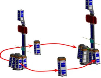
of various components of a modular telescope system, which will be demonstrated on the AAReST

[image:11.595.236.406.522.653.2]

(Autonomous Assembly and Reconfiguration of a Space Telescope) mission (see Figure 1.1).

Figure 1.1: Concept for AAReST mission reconfigurable space telescope.

The problem of accurately and robustly modeling the dynamics of a self-assembling system presents

(12)

several challenges which, while also present in other types of systems, play a predominant role in the

dynamics of the systems of interest. For example, the dynamics to be modeled include collisions,

sustained contact (i.e. clumping or jamming), and complicated multiple-contact scenarios between

stiff or rigid bodies. A general model also needs to account for non-smooth non-convex bodies and

strong attractive forces at contact interfaces between bodies.

In addition to the problem of modeling the dynamics, the design and certification problems for this

type of system present novel challenges in their own right in the areas of robust and optimal control,

and model-based system design and certification. These problems take on several flavors for active

and passive systems. For passive systems, one can think of controlling the dynamics to affect a

desired final configuration via the design (geometry, inertial properties, potentials) of the modules

themselves, subject to uncertainty. For active systems, control algorithms must be formulated to

avoid contact between non-smooth bodies or to account for the fact that contact interactions will

play a role in the dynamics. For computational studies of passive systems, an accurate description

of the mechanical system including contact interactions is essential. In the case of active systems,

a method of controller design that explicitly accounts for the non-smooth nature of the system is

required.

Before moving on to a more detailed overview of how these challenges are met, it is worth

not-ing that they are not unique to self-assemblnot-ing systems. However, the extent to which they are

present motivates the need for new tools to model, design, and better understand self-assembling

systems, with the added benefit that, once developed, these tools become directly applicable to

Overview

This thesis is organized as follows. In Chapter 2, a novel approach to robust fine-scale collision

detection for non-smooth polyhedral bodies is presented. This approach, which is called the

Sup-porting Separating Hyperplane algorithm (or simply the SSH algorithm), is based on fundamental

separation theorems for convex sets. It is shown that for polyhedral sets, the SSH algorithm may

be evaluated as a linear program (the SSH LP), and that this linear program is always feasible and

always subdifferentiable with respect to the configuration variables, which define the constraint set

of the linear program. This is true regardless of whether the program is primal degenerate, dual

degenerate, or both. The subgradient of the SSH linear program always lies in the normal cone of the

closest admissible configuration to an inadmissible contact configuration. In particular if a contact

(13)

imations. In the final category, a parameter-free explicit contact algorithm for rigid body dynamics

is developed for smooth or non-smooth geometries within the framework of a constrained variational

integrator. This algorithm extends the decomposition contact response (DCR) algorithm for finite

element dynamics of Cirak and West [15], and can be considered an explicit approximation to the

fully implicit (exact) variational approach of Fetecau et al. [25]. For non-smooth bodies, collision

detection and accurate momentum updates are enabled by the supporting separating hyperplane

SSH algorithm.

With robust collision detection and simulations methods in hand, in Chapter 4 these concepts

are combined and incorporated into optimal control problems with both collision avoidance and

planned contacts between non-smooth bodies. This chapter is divided into two main sections. In

the first, the structure preserving constrained optimal control methodology for discrete mechanical

systems (DMOCC) introduced in Leyendecker et al. [52] is extended to include collision avoidance

and planned contacts. The latter goal is accomplished without over-constraining the problem by

allowing the physical contact time(s) and configuration(s) to vary in the course of the optimization.

The final sections of both Chapters 3 and 4 summarize the application of the methods developed

therein to real-world design and control problems of the AAReST mission.

As mentioned in the motivation for this work, the problems inherent in modeling and designing

self-assembling systems are not necessarily unique to this type of system; it follows that the tools

developed in this thesis can naturally be extended to enrich other fields. To this end, future research

directions related to and inspired by the work presented in this thesis are presented in Chapter 5

(14)

2

Non-Smooth Collision Detection

2.1

Introduction

In this chapter, a contact detection algorithm for non-smooth convex bodies is developed. The

pro-posed contact detection algorithm can be concisely described as a supporting separating hyperplane

(SSH) test for interpenetration, and is based on standard separation theorems for compact convex

sets. The test is developed in detail for polyhedral bodies, where the SSH test can be effectively

reformulated as a linear programming problem–the SSH LP. It is further shown that the subgradient

of the SSH LP can be readily evaluated and–as will be discussed in detail in future chapters–that

the subgradient supplies the force system at the time of contact.

2.2

Background and Related Work

2.2.1

Previous Work

A large body of literature exists on the efficient detection of collisions, driven in large part by

advances in computational geometry, computer graphics and robotics (see Akgunduz et al. [2], Aliyu

and Al-Sultan [3], Chakraborty et al. [13], Chung and Wang [14], Cohen et al. [17], Dobkin and

Kirkpatrick [20], Ericson [22], Gilbert et al. [29], Gilbert and Hong [30], Gottschalk et al. [33], Li

et al. [54], Lin et al. [56], Tang et al. [81]). While several advances have taken place in the past several

years, the 2001 review by Jimenez et al. [36] and the 2005 book Ericson [22] effectively summarize

the essential state of the art. The development of the SSH algorithm follows the same track as much

of this literature, which develops collision detection algorithms for use with convex polyhedra and

for solid models that have been discretized by polyhedra. However, the collision detection algorithm

presented here is general enough to extend to an interpenetration test between any two smooth or

(15)

can quickly compute candidate areas for contact, and refine those areas to determine which simplices

are actually involved in a collision. However, when the objects get close enough for the bounding

volumes to suggest that contact might have taken place, a finer detection test must be used to

conclusively declare that a collision has taken place. Another option that works on the coarse and

fine levels, proposed by Chung and Wang, detects collision based on the existence (or not) of a

separating vector [14]. While the present interpenetration function is universal and robust, in that

it can be evaluated for any pair of convex bodies, and is certainly capable of serving as a coarser

scale collision detection test, one would rather suggest its use as a final test in conjunction with one

of the coarser tests referenced here.

The interpenetration function here can be seen as an alternative to the heuristic search for a

sepa-rating vector developed by Chung and Wang [14], and also as a an alternative to other linear

pro-gramming approaches such as those proposed by Akgunduz and others [2] and Aliyu and Al-Sultan

[3], to which Seidel [77] made key contributions. The advantage of the proposed linear

program-ming approach to collision detection is that it provides extremely useful additional information for

physics-based dynamics simulations and closest-point projection (CPP) operations. In the present

work, a well known path to collision detection and undertaken in the form of a search for a separating

vector. However, this search for this vector si conducted in an optimal way so that it always lies in

the normal cone of the closest admissible configuration to an inadmissible contact configuration and

respects any symmetries present in the geometry of the contact configuration. Furthermore, unlike

previously proposed methods, the present approach ensures that the subgradient of the SSH linear

program is only non-zero with respect to degrees of freedom directly involved in the collision and

also respects the geometry of the contact configuration. For example, if a contact surface exists, the

subgradient is orthogonal to the contact surface.

2.2.2

A Motivating Example

The aforementioned useful additional information is the key motivation for this work. By way of illustration, a widely accepted treatment of contact in the equations of motion may be considered:

the introduction of a contact potential into the action functional. This potential takes the form of the

indicator function,IAof a setA ⊂ Qcontaining all admissible (non-interpenetrating) configurations

(16)

varibles consist of configurations q _{∈ Q} and velocities ˙q _∈ TqQ (see Cirak and West [15], Clarke

[16], Fetecau et al. [25], Gonzalez et al. [32], Kane et al. [38], Leyendecker et al. [50], Pandolfi

et al. [68] and additional details in Chapter 3). For simplicity in the present example, both_Q and

TqQ will be associated with Rn. Admissible (non-contact) configurations for q occupy the subset A ⊂ Q.

In the absence of other potentials and external forces, the action functional reads

I(q) =

Z T

0 L

(q,q˙)dt, (2.1)

for the Lagrangian

L(q,q˙) = ˙qT_M_q_˙

−I_A(q), (2.2)

whereM is an appropriate mass matrix and

IA(q) =



 

 

0 ifq∈ A ∞ otherwise

. (2.3)

The equations of motion can be recovered by requiring stationarity of_I

Mq¨+∂IA(q)30. (2.4)

In (2.4), ∂I_A(q) denotes the generalized differential of the indicator function (c.f. [16, 38]). It is readily shown that the generalized differential of the indicator function of a set is given by the normal

cone,NA, of the set

∂I_A(x) =N_A(x). (2.5)

It follows from (2.4) that the contact forcesfconare related to the normal cone by:

fcon∈ −NA(q). (2.6)

The normal cone is defined precisely in Section 2.3 of this paper. For this introductory example it

(17)

Where_L(q,q˙) is the same as the expression in (3.34). In this case, the equations of motion at the time of contact read as jump conditions on the change of momentump=Mq˙ and kinetic energy during the collision

pT_M−1_ptc+

tc− = 0 (2.8a)

[[p]]tc+

tc− ∈NA(q(tc)). (2.8b)

Equations (2.8a) and (2.8b) describe the conservation of energy and momentum during the collision,

respectively. In practice, the restriction that the forces from (2.6) and the change in momentum in

(2.8a) be in the normal cone of the admissible set are accomplished by constraining the configuration

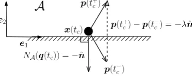
variables to be in _{A ⊂ Q} via an interpenetration function g(q) that is negative if two bodies are not overlapping and positive if they are, that is _A = _{q_{∈ Q|}g(q)_≤0_}. For example, consider a point mass in two dimensions (i.e., q = (q1, q2)) falling onto a flat surface coincident with the e1−axis (see Figure 2.1). In this case, the admissible set of configurations for the mass are described

by _A =

q_∈R2| h−nˆ,qi ≤0 with q = (q1, q2) and ˆn = (0,1)T, and the normal cone of the

admissible set has the unique values NA(q) =−nˆ if q2 = 0, NA(q) =0if q2 >0 and NA(q) =∅

otherwise.

In this case, (2.8a) can be expressed as [15]

[[p]]tc+

t_c− =λ∇g, (2.9)

which for our example is equal to

[[p]]tc+

t_c− =−λnˆ (2.10)

ifq2= 0. Here,λ∈Ris a scalar parameter (see [15] for details). The simplest re-expression of (2.6)

(18)

IA(q)≈VA(q) =



 

 

0 ifg(q)<0 C

2g(q)2 otherwise

, (2.11)

whereC_∈Ris a constant. This leads to the formulation

fcon=−∇VA(q), (2.12)

which for the point-mass example is

fcon=



 

 

0 ifg(q)<0

−C_h−nˆ,q_inˆ otherwise

. (2.13)

This simple example lends itself to a straightforward geometric interpretation of NA = ∂IA, in

that the contact forces must be normal to the contact surface (see (2.12)) and that the change of

momentum must also be normal to the surface (see (2.9)). Thus, to accurately conserve momentum

and approximate the continuous equations of motion, a constraint function g(q) should have the property that_∇g(q)_≈NA(q), as in the point-mass example.

x(tc)

p(t−

c)

e2

e1

A

NA(q(tc)) =−nˆ

p(t+

c)

p(t+

[image:18.595.227.422.418.495.2]

c)−p(t−c) =−λnˆ

Figure 2.1: A point mass striking a flat, frictionless surface in the absence of external forces and potentials. In this example,λ= 2h−nˆ,p(t−c)i.

Some time integration schemes based on Lagrangian mechanics use a contact potential in the action

functional and require a continuous interpenetration function that is at least sub-differentiable [15,

25, 32, 41, 50]. Such a potential is easy to construct for models of geometrically simple bodies

and admissible configurations, but a good choice for this potential is much less obvious for complex

geometries.

The preferred function for use in these applications has been a test for overlapping oriented simplices

(OOS); i.e. tetrahedra in three dimensions, and triangles in two dimensions (c.f. [15, 38]). The OOS

test can accurately provide a functiong(x), which indicates whetherIA(q) is zero, but it is obvious

(19)

composed of these simplices. Thus, the OOS test is inadequate in particular for systems that do

not have the capacity to absorb these spurious forces through deformations or motions; for example,

in crowded or tightly-packed systems, stiff systems, and rigid body dynamics an accurate gradient

∇g(q)≈NA(q) is essential.

The OOS test has another key shortcoming. Before it can be evaluated, the algorithm must first

determine whether the two segments or triangles of interest are indeed overlapping. Other versions

of the test call for determining the type of contact first (face-edge, face-corner, face-face). These

different ‘switches’ that precede the actual evaluation of the OOS test are particularly cumbersome

when the time-integration algorithm is implicit or calls for optimization to resolve the contact

con-figuration as they amount to changing the potential energy function or contact constraints as the

algorithm is trying to converge.

In contrast, the supporting separating hyperplane (SSH) algorithm which is outlined in Algorithm

1 in Section 2.7 compares favorably to the OOS approach because 1) it is global in that it considers

whole bodies and it does not require any ‘switches’ or additional calculations to classify types of

contact that have taken place, and 2) it always supplies a gradient direction in the normal cone

of the contact configuration, i. e., the closest admissible configuration to the present inadmissible

configuration. Furthermore, the force system described by _−∇V_A(q) in a contact configuration is local to the features on each body involved in the collision. Finally, the dual solution to the SSH

linear program can be used to determine closest-feature information and to determine an excellent

approximation to the exact point of contact.

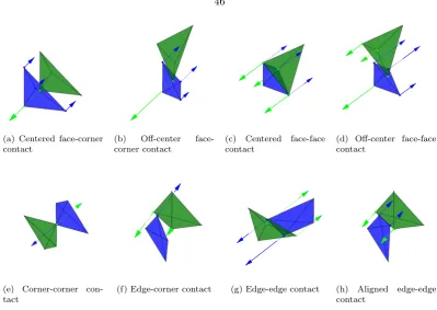
(a) OOS function gradient (b) SSH function gradient

(20)

2.2.3

Organization

The development of the SSH algorithm, including the derivation of its subderivative is illustrated in

the workflow diagram in Figure 2.3. The algorithm is based on concepts and theorems from convex

and affine geometry, and can be reduced to a quadratically constrained linear program (QCLP) for

polyhedral bodies with isolated extreme points. However, the structure of this QCLP is such that an

equivalent linear program (LP) can always be formulated. Due to the nature of linear programming,

an explicit expression of the subderivative of the SSH LP can be derived, which can then be used in

various applications.

Separation Theorems, Signed Distance Function

Convex Geometry, Affine Geometry, Hyperplanes General SSH Test (any convex bodies)

SSH QCLP for Polyhedral Bodies SSH LP for Polyhedral Bodies

Affine Geometry, Finite Extreme Points QCLP Properties Explicit Formula for SSH LP Subderivative

Solution Structure of Linear Programs Applications Using SSH LP+Subderivative

Figure 2.3: Work flow pyramid for the development of the SSH algorithm and the explicit derivation of its subderivative. Items in between levels are features of the lower level which allow progression from the lower level to the upper level.

The organization of this chapter is as follows. In Section 2.3, the basics of hyperplanes and affine

geometry are reviewed, including key separation theorems for convex sets, which are used in Section

2.4 to develop the SSH test for interpenetration and prove that the algorithm always accurately

indicates whether or not two convex sets are separable. In Section 2.4, it is shown that for polyhedral

sets, the algorithm can always be formulated and solved as a feasible linear program. Section 2.5

reviews the solution to a linear program based on the primal simplex method that is used in Section

2.6, where nonsmooth analysis is used to expand on the results of Freund [27] and Freund [26]

and derive an explicit analytical expression for the subderivative of a linear program in extended

standard form. The implementation of our method is discussed in Section 2.7. Finally in Section

2.8, the effectiveness of our function in determining the e features involved in a collision and an

(21)

we refer the reader to these resources for precise definitions of bounded, closed, and compact sets,

and the convex hull of a set. For this and the following sections, unless otherwise stated, we denote

the inner product between two vectors inRn as h·,·i, the Euclidean norm of a vector inRn as k·k,

and the cardinality of a set as_{| · |}.

2.3.1

Affine Sets

A subsetM _⊂Rn is called an affine set if for everyx∈ M, y ∈M, andλ∈R, (1−λ)x+λy∈

M.

2.3.2

Convex Sets

A subsetC_⊂Rnisconvexif for all distinct pointsx∈C,y∈C, and all 0≤λ≤1, (1−λ)x+λy∈C.

Clearly, all affine sets are also convex sets.

2.3.3

Hyperplanes

Following [34], we use the notationHα,a for the hyperplane inRn, with α∈Rn and a∈R, as the

set of points such that

Hα,a:={x∈Rn| hα,xi −a= 0}, (2.14)

which is an affine (and convex) set. It is recognized that αis the normal vector to the plane, and that Hα,a has two distinct sides. An equivalent (point-normal) representation, withα ∈ Rn and

a_∈Rn, is

Hα,a:={x∈Rn| hα,x−ai= 0}, (2.15)

where we can identify a=_hα,a_i. For any choice of α and a, the hyperplane associated with µα

(22)

restrictα_∈Sn−1_{. Thus, for the signed distance between a point}_y

∈Rn and a hyperplane, we use

the notation

Hα,a(y) :=hα,yi −a. (2.16)

The definition of parallel hyperplanes can be further restricted to denote two hyperplanesHα,aand

Hµα,b for which µ = 1. Thus, the signed distance from Hα,a ≡ Hα,a to Hα,b ≡ Hα,b is given

by

d(Hα,a, Hα,b) =d(Hα,a, Hα,b) =b−a, (2.17)

where the equivlance of the hyperplanes is due toa=_hα,a_iandb=_hα,b_i, respectively.

2.3.4

Construction of Convex Sets

2.3.4.1 Intersection of Half-Spaces

Let the(closed) half-spaces associacted with a hyperplaneHα,a be defined as

Hα+,a:={x∈Rn|Hα,a(x)≥0} (2.18a)

Hα−,a:={x∈Rn|Hα,a(x)≤0}. (2.18b)

It may readily be shown that the intersection of convex sets is also convex (c.f. Theorem 2.1 in [75]).

Thus, the following setK is convex (and closed)

K=∩ {x∈Rn|Hαi,ai(x)≤0, i= 1. . . j}. (2.19)

If K 6= ∅ and j → ∞, then some portion of the boundary of K (bdK) is said to be smooth.

Furthermore, K is a compact set if it is bounded. For finite j, K as defined above is non-smooth

and is called a polyhedral set. In the case that a polyhedral set is bounded (and therefore compact),

it may alternately be called a polytope inRn or simply a polyhedral body (also inRn), in reference

(23)

For a compact set, extK ₆=_∅, and all extreme points of K are on bdK. Thus, a set K, which is

convex and compact in Rn, can alternately be described as the convex hull of its extreme points,

K= co(extK). By this construction, for a finite number of extreme points,K is a polytope. This

allows the description of all points inKas a convex combination of its extreme points. That is, for

allx∈K,y∈extK, andλi>0,

x=

|extK|

X

i

λiyi, where:

|extK|

X

i

λi= 1.

(2.20)

For a polyhedral set, the set of vertices is equal to the set of extreme points.

2.3.5

Supporting Hyperplanes

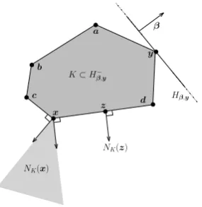
A hyperplaneHα,ais said to support the setKwhenKis entirely contained in eitherHα+,aorHα−,a, and bdK_∩Hα,a6=∅. It is said to supportK atx∈K when, in addition,x∈Hα,a.

2.3.6

Normal Cone to a Convex Set

For the following analysis, it suffices to present a normal cone definition that is strictly relevant to

convex sets. However, it is important to note that the idea can be extended to non-convex sets and

is important in non-smooth analysis (see Clarke [16] for additional information). The normal cone

NK(x) to a convex set K at the point x∈K may be defined as the set of directions ν ∈Rn for

whichKis in the negative halfspace ofHν,x, i.e.

NK(x) ={ν∈Rn|Hν,x(x∗)≤0 ∀x∗∈K}

NK(x) =

ν_∈Rn|K⊂Hν−,x .

(24)

Thus, it is obvious that NK(x) will contain more than one directionν when Kis a polyhedral set of dimension nin Rn ifxis in a feature of K of dimension less thann−1. Figure 2.4 shows two

examples of normal cones.

K⊂H− β,y

NK(x) x

Hβ,y β

y

NK(z) z a

b

[image:24.595.255.398.131.278.2]

c _d

Figure 2.4: Schematic of concepts for hyperplanes and convex sets for a compact polyhedral set, K. Pointsa,b,c,x,d,y form the set of extreme points of K, and z is not an extreme point. The hyperplaneHβ,y supports the setK at ysuch that K⊂Hβ−,y. The normal cone of K is shown at

two points: x_∈extK whereNK(x) is not unique, andz_∈/extK whereNK(x) is unique.

As it will be useful later, it is noted here that for convex sets there is a one-to-one correspondence

between finding a hyperplane supporting a set at a given point, and finding a direction in the normal

cone at the point.

2.3.7

Separation of Convex Sets

Thestrictseparation of sets is defined as follows: for two non-empty closed convex sets,K1andK2

for whichK1∩K2=∅andK2 is bounded, there existsαsuch that:

sup

y∈K2

hα,y_i< min

x∈K1h

α,x_i. (2.22)

Furthermore, ifK1 is also bounded, then there existsαsuch that

max

y∈K2h

α,y_i< min

x∈K1h

α,x_i. (2.23)

(25)

In other words, a vectorαis a separating vector if it can be associated with a hyperplaneHα,a that properly classifies all of the pointsK1and K2 such thatK1⊂Hα+,aand K2⊂Hα−,a. The converse is also true. For two compact convex sets, if α cannot be found such that maxy∈K2hα,xi ≤ minx∈K1hα,yi, thenK1∩K26=∅. Figure 2.5 illustrates the definition of proper (α) and strict (β) separating vectors, along with examples of hyperplanes associated with these vectors.

K1

K2

Hα,a

Hβ,b

α β

Figure 2.5: An example of strictly separable sets. The vector β and associated hyperplane Hβ,b strictly separateK1andK2, whereas the vectorαand associated hyperplaneHα,aproperly separate K1andK2. Note that the hyperplane drawn labeledHβ,bis not a unique choice for the vectorβ.

2.4

Supporting Separating Hyperplane Algorithm

In this section, the Supporting Separating Hyperplane (SSH) algorithm as a test for interpenetration

is developed. To begin, the algorithm is developed for general compact convex sets as a constrained

optimization problem with a linear objective function. It is then shown that, for compact polyhedral

sets, the algorithm can always be reformulated so that all constraints are linear, i.e., as a linear

programming problem.

To begin, let _{Hα,a}+_K₁ be defined as the set of supporting hyperplanes of K1 at x∈ bdK1 such

that K1⊂Hα+,a and{Hβ,b}−_K₂ be defined as the set of supporting hyperplanes ofK2 aty∈bdK2

such that K2 ⊂Hβ−,b. Again, all normal vectors of {Hα,a}+K1 and {Hβ,b}

−

K2 are unit vectors (i.e.,

α,β _∈ Sn−1_{). Define the function ˜}_h₍_K

1, K2) as follows, where the function d(Hα,a, Hα,b) was

(26)

˜

h(K1, K2) = max

Hγ,a¯∈{Hα,a}+K1 H_γ,¯b∈{Hβ,b}−K2

d(Hγ,¯a, Hγ,¯b) (2.25)

The solution to (2.25) is the maximum signed distance between parallel supporting hyperplanes of

each set, with the restriction that each hyperplane properly classify its associated set.

Remark 2.1. From the point-normal description of a hyperplane, for two non-empty compact

con-vex sets, ˜h(K1, K2) = ˜h(extK1,extK2). Since d(Hα,a2, Hα,a1) = d(Hα,a2, Hα,b1) ∀b1 −a1 ∈ Hα,a1, i.e., b1−a1 ∈Hα,a1 ⇒Hα,a1∩Hα,b1=Hα,a1 =Hα,b1. Therefore, if Hα,a1 supportsK1

ata1∈/extK1, there is an equivalent hyperplane that supportsK1 atb1∈extK1, and

˜

h(extK1,extK2) = ˜h(K1, K2). (2.26)

Remark 2.2. The problem (2.25) is always feasible. For two compact, convex sets, one can always

find two parallel supporting hyperplanes such thatHα,a1 ∈ {Hα,a} +

K1 andHα,a2 ∈ {Hβ,b}

−

K2. This

remark is obvious ifK1∩K2=∅, and at least one hyperplane exists that strictly separatesK1 and K2. To show that this is true if K1∩K26=∅, consider a plane Hβ,b that properly separates two sets

for which maxy∈K2hβ,yi= minx∈K1hβ,xi, and K1 and K2 uniquely properly separable. Because

the sets are compact and convex, such a plane can always be found. Further, define two equivalent planes for whichHβ,b2(y∗) = 0for somey∗∈bdK2andHβ,b1(x∗) = 0for somex∗∈bdK1. If one

now setsb2=hβ,y∗iandb1=hβ,x∗iand undertakes a translation ofK2 and, by extension,Hβ,b2

by β so that b2 =hβ,y∗+βi, K1 and K2 no longer are separable, but two parallel hyperplanes

that are in the domain of (2.25) are retained. The cases discussed in this remark are illustrated in Figure 2.6.

K1 K2

α Hα,a1

Hα,a2

(a) Strictly separable sets

β Hβ,b

y∗

x∗

(b) Properly separa-ble sets

β Hβ,b1

y∗₊_ǫ_β

x∗

Hβ,b2

(c) Non-separable

sets

Figure 2.6: Figures 2.6a through 2.6c illustrate the cases discussed in Remark 2.2. One of the many possible sets of supporting hyperplanes in the domain of (2.25) is shown for strictly separable sets in Figure 2.6a. In Figures 2.6b and 2.6c, the circular set remainsK1, and the triangular set remains K2, but they are not explicitly labeled to simplify the drawing. Figure 2.6b shows a hyperplane

(Hβ,b) which is clearly in the domain of (2.25), and two arbitraily chosen points,x∗ ∈bdK1 and

y∗_∈_bd_K

2, at whichHβ,bsupports each set, as described in Remark 2.2. Finally, Figure 2.6c shows the translation ofK2 byβ, and the corresponding hyperplanes in the domain of (2.25).

Before proceeding, a constrained optimization problem overα∈Sn−1_{, and}_a

(27)

extK1⊂Hα+,a1

extK2⊂Hα−,a2.

(2.27)

Theorem 2.1. Two compact convex sets K1 andK2 are strictly (properly) separable if and only if h >(≥)0.

Proof. It is first shown that h > 0 ⇒ K1∩K2 = ∅, and by extension that h = 0 implies that K1 andK2 are properly separable. From the definition of a supporting hyperplane, a1≤ hα,xifor

x∈extK1and likewisea2≥ hα,yifory∈extK2. It follows from the constraints in equation (2.27)

that maxa1 = minx∈extK1hα,xi and that mina2 = maxy∈extK2hα,yi at the solution. Therefore,

we can do a portion of the optimization explicitly and see that

h(K1, K2) = max

α∈Sn−1

x∈extK1

y∈extK2

a1(α,x)−a2(α,y)

= min

α∈Sn−1

x∈extK1

hα,x_{i −} max

α∈Sn−1

y∈extK2

hα,y_i,

subject to the same constraints as (2.27). From the definition of strict (proper) separation of sets, if α can be found such thath(K1, K2)>(≥)0, thenK1 andK2 are strictly (properly) separable, thus h >0_⇒K1∩K2=∅, and that h= 0⇒K1∩K2⊂Hα,a1≡Hα,a2.

To show thath >0⇐K1∩K2=∅, note that the domain has been restricted such thatHα,a1 properly

classifies K1 ⊂Hα+,a1, and Hα,a2 properly classifies K2 ⊂Hα−,a1. In this domain, the maximum

distance a1−a2 is positive (non-negative) only if, in addition, K2 ⊂ Hα−,a1, and K1 ⊂H +

α,a2, in

which case, by the definition of strict (proper) separation of sets, α is a separating vector and both hyperplanes are separating hyperplanes. Therefore h >0_⇐K1∩K2=∅, andh= 0⇐K1∩K2⊂

Hα,a1 ≡Hα,a2.

Corallary 2.2. Corallary to Theorem 2.1 Two compact convex sets K1 andK2 are not separable if

and only ifh <0.

Proof. Follows directly from Theorem 2.1.

(28)

K1

K2

d <0

α

Hα,a1 Hα,a2

(a)

K1

K2

d >0

α Hα,a1

Hα,a2

(b)

K1

K2

maxd >0

α∗ Hα∗,a∗

2 Hα∗,a∗

1

(c)

K1 K2

d <0

α

Hα,a1 Hα,a2

(d)

K1 K2

d <0

α

Hα,a1 Hα,a2

(e)

K1

K2

maxd <0

α∗ Hα∗,a∗

1 Hα∗,a∗

2

[image:28.595.211.425.58.400.2]

(f)

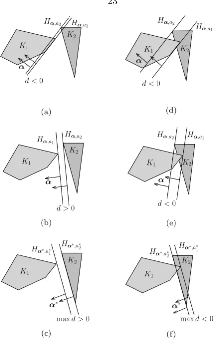
Figure 2.7: Figures 2.7a through 2.7c show the domain ofpotentially separatingsupporting hyper-planes for two separable polyhedral sets. The sign ofddenotes whetherHα,a1is in front of (positive) or behind (negative)Hα,a2 according to the direction ofα. Figures 2.7d through 2.7f show the same domain for sets that are not separable.

2.4.1

Formulation as a Quadratically Constrained Linear Program

Equation 2.27 can further be refined by transforming the restriction on the domain to constraints

on the solution vector according to the definition of a supporting hyperplane as follows:

h(K1, K2) = max

α∈Rn

a1,a2∈R

a1−a2, Subject to:

hα,x_{i −}a1≥0, x∈extK1 hα,yi −a2≤0, y∈extK2 hα,α_i= 1.

(2.28)

(29)

2.4.2

Interpenetration Detection as a Linearly Constrained Linear

Pro-gram

The goal of this section is to formulate a linear program (LP) which, like (2.28) indicates whether

or not two sets are intersecting when the sets K1 and K2 are both compact polyhedral sets. To

begin, we note that the structure of (2.28) is linear in the objective function, and in all of the

constraints with the exception of the final constraint, that _hα,α_i = 1. For the purposes of this analysis, consideration will be restricter to sets for which dim(K1) = dim(K2) =n, i.e. sets of the

same dimension of the space in which they are embedded, however the results may be extended to

some cases in which dim(K1) < n and/or dim(K2)< n. The following remarks will be useful in

showing that the solution to a linear program of the form

g(K1, K2) = max

α∈Rn

a1,a2∈R

a1−a2, Subject to:

hα,xi −a1≥0, x∈extK1 hα,y_{i −}a2≤0, y∈extK2 hβ,αi= 1,

(2.29)

for certain choices of β is equivalent to (2.28), in that a solution vector, a = (αa1 a2) to the

quadratically constrained program (the QCLP, or simply QP) is equal to a solution to the linearly

constrained program (the LP) normalized by_kα_k.

Remark 2.3. For two compact convex sets,K1 andK2, if K1∩K2 =6 ∅, then d(Hα,a1, Hα,a2)≤ 0∀Hα,a1 ∈ {Hα,a}

+

K1, Hα,a2 ∈ {Hα,a}

−

K2. This follows from Theorem 2.1 due to0≥maxd(Hα,a2, Hα,a2)≥ d(Hα,a2, Hα,a2).

Remark 2.4. If two compact, convex sets are separable withdim(K1) = dim(K2) =n, then there

is a compact set of directions α ∈ Sn−1 which render the QP (2.28) non-negative. This follows from the observation that there is a compact set of points inbdK1 andbdK2at which a separating

hyperplane can support each set. Furthermore, with the restriction that dim(K1) = dim(K2) =n,

this set will be contained in less than a hemisphere ofSn−1_{. This set of separating directions will be}

(30)

K1⊂Hα+,x, K2⊂Hα−,y, x∈bdK1, y∈bdK2}⊂Sn−1. An example of S(K1, K2)for two sets in

R2 is shown in Figure 2.8.

K1

K2

Sn−1

α1 α2

S(K1, K2)

Figure 2.8: The left schematic highlights the set of points in bdK1 and bdK2 at which each set can

be supported, along with several pairs of supporting hyperplanes satisfying the constraints of (2.28). In the right schematic, the setS(K1, K2) of separating directions for the two bodies sketched in the

left schematic is shown.

Remark 2.5. The QP (2.28) always has a finite solution so long as allxi, andyi are finite. This

follows from 1)the observation that the objective function only has a non-zero gradient in thea1−a2

subspace, and 2)the structure of the first two sets of contraints establishes an upper bound for a1,

and a lower bound fora2 for anyα. Thus, the objective function is always bounded in its increasing

direction for anyα_∈Sn−1_{, as can be seen in Figure 2.9.}

a

1

a

2

Increasinga1−a2

a1−a2= 0

K1

K2

K1

K2

α α

Figure 2.9: The level sets of the objective function, a1−a2, are shown. Schematics of the upper

bound for a1 and the lower bound for a2 are shown for selected directions α which are feasible

solutions to (2.28), sketched in the correponding diagrams superimposed on the plot.

(31)

hα,y_{i −}a2≤0, y∈extK2 hα,β_{i −}1 = 0.

The inner optimization problem then amounts to an optimization over (a1, a2) for a fixed vector

α = ¯β, which is always a bounded, feasible problem according to the preceeding remark. Thus, removing the constraint thatα_∈Sn−1 _{will result in a problem with at least one feasible solution for}

any β.¯

With these preliminaries established, call a1−a2 = γ a feasible solution to the QP (2.28), and

a∗

1−a∗2 = γ∗ an optimal solution to the QP. The corresponding equivalent solutions to the LP

(2.29) will have the valuesγ_kαLPkandγ∗kα∗LPk, respectively, withαLP satisfyingHβ,1(αLP) = 0. Futhermore, we will use the notationa= (a1, a2) to denote the solution to the QP (2.28) is thea1−a2

subspace, and aLP the corresponding solution to the LP (2.29), with the relationship a= _k_αaLP_LP_k. Before proceeding with the key theorem of this section, recall the definition of the set of separating

vectors for the sets given in Remark 2.4 asS(K1, K2) =α∈Sn−1|K1⊂Hα+,x, K2⊂Hα−,y,

x_∈bdK1, y∈bdK2} ⊂Sn−1, which will be equal to the empty set ifK1 andK2are not

separa-ble.

Theorem 2.3. An optimal solution, a∗LP, to (2.29) is equivalent to an optimal solution, a∗QP, to

(2.28) for a given choice of β_∈Sn−1 _{if the following statements hold.}

i The open hemisphere of Sn−1 centered onβ contains of _S(K1, K2)andα∗QP.

ii For all other feasible solutions to the linear program,aiLP,sign(γi)6= sign(γ∗),

αi_LP

<

γ∗kα∗LPk

γi −1

+ 1 forγ

∗ _>₀_{, or} αi_LP

>

γ∗kα∗LPk

γi −1

+ 1 forγ

∗ _<₀_.

Proof. Proof of Theorem 2.3

By statement (i), the solution direction α∗

QP has an equivalent solution direction αLP ∈ Hβ,1.

Also by statement (i), as _kα_{k → ∞}, γ becomes negative for directions α _∈ Hβ,1, so all feasible

solutions to the LP are bounded from above. It is still possible for another feasible solution direction, α0

LP ∈ Hβ,1, of the linear program to satisfy γ0 α0_LP

> γ∗kα∗_LPk, with γ0 < γ∗. Trivially, if

sign(γ0₎

6

= sign(γ∗₎_{, then} _α∗

(32)

can calculate the point, acrit, at which the ray a2 = a 0 2 a0

1a1

(with a0 _{= (}_a0

1, a02)as components of the

corresponding feasible solution to (2.28)) intersects the level seta1−a2=γ∗kα∗LPkas

acrit= γ

∗_k_α∗

LPk γ0 a

0

It then follows fromα0_LP =k

a0LP−a

0

k

ka0_k + 1 that

α0_LP

<kαcritk ⇒γ0

α0_LP

< γ∗kα∗_LPk forγ∗>0,

and

α0_LP

>kαcritk ⇒γ0

α0_LP

< γ∗kα∗_LPk forγ∗<0,

with_kαcritk=

γ∗kα∗LPk

γ0 −1

+1, which is the final condition in statement (ii).

In practice, choosing a vectorβa priori to meet the first requirement of Theorem 2.3 is not hard to do, in particular as the optimal QP solution decreases to zero or becomes negative and _S(K1, K2)

shrinks to the empty set, which renders (i) less and less restrictive. We will not present a concise

result on this topic, although we note that _S(K1, K2) could be explicitly calculated and a central

direction in this set chosen if needed to ensure that (i) is met so that the optimal LP solution is

bounded. Furthermore, if an unbounded LP is encountered–which in itself implies that the sets are

separable–β can simply be reset based on the unbounded direction, and the new problem solved to determine a separating direction.

Perhaps more importantly, choosingβ to meet the second requirement of the theorem is actually not essential to determine whether or not two sets are separable, or even to resolve a separating

direction if they are. By Remark 2.3, if K1 and K2 are not separable, then any choice ofβ will

indicate this fact, by rendering the objective function of the LP (2.29) negative. However, it is

possible to selectβ which gives a ‘false positive’, for which the solution to the LP is negative, but the solution to the QP is positive, implying that condition (i) in Theorem 2.3 has not been met. To

avoid this,βshould be initially selected so thatβ and some subset ¯_{S ⊂ S}(K1, K2) are in the same

open hemisphere.

In other words, one does not need to find an equivalent LP solution to the QP (2.28) in order to obtain an accurate result for the SSH test using a linear program. Rather, one simply needs to solve

(33)

2.5

Linear Programming

For completeness, this section provides a brief review of the well-studied topic of optimality

con-ditions and solution strategies for linear programs (Dantzig and Thapa [19] provides a thorough

primary reference). While this will likely be a review for many readers, the formulation of the

problem is essential to the evaluation of its SSH linear program’s subderivative.

To simplify notation in this section, the number of inequality constraints in a linear program whill

be denoted asm1, the number of equality constraints asm2, and the number of primal variables is

n. All vectors are to be understood as column vectors and are denoted by bold lowercase letters, for

examplea_∈Rn. The combination of two vectorsa1 ∈Rn1 anda2 ∈Rn2 into an extended vector

a _∈Rn1+n2 is denoted, with a slight abuse of notation, asa =

a1 a2

. Subscript notation such

as ai denotes theithcomponent ofa. Matrices such asA∈Rm×n are denoted by bold uppercase

letters, and the combination of matrices of compatible dimensions into entries in block matrices is

denoted by means of square brackets, e.g. hA1 A2 i

. Subscript notation such asAij denotes thejth

component of theith _{row of}_A_.

2.5.1

Conditions for Optimality

Linear programs of the following form will be considered

F(A,b,c) = max

x∈Xc

T_x

with:X ={x∈Rn|A1x≤b1,A2x=b2,x≥0},

(2.30)

for which X is a set of feasible solutions to the (primal) problem (2.30). Later, X∗ _⊂ _X _will

be defined as the set of optimal primal solutions to (2.30). In this problem, the total number of

constraints is m =m1+m2, and A1 ∈Rm1×n_, _A

2 ∈ Rm2×n_{, with} _b

1 and b2 also of compatible

dimensions. Alternately, the notation thatAT ₌h

AT1AT2 i

, andb=b1b2

will be adopted.

(34)

From the primal problem (2.30), the Lagrangian function can be written as

LP(x,λ,µ) =cTx−λT1(A1x−b1)

−λT2(A2x−b2) +µTx,

(2.31)

where λ =λ1 λ2

and µare lagrange multipliers. The Karush-Kuhn-Tucker (KKT) conditions that are necessary for optimal primal (x∗_{) and dual (}_λ∗_{) variables are}

x∗_∈X

λ∗T

1 (A1x∗−b1) = 0,

x∗T c₋ATλ∗

= 0,and

ATλ∗_≥c, λ∗1≥0,

where the ith _{constraint is said to be active if} _λ

i 6= 0. This corresponds an inequality being an

equality at the solution.

To state the dual program to (2.30), we first set y = y1 y2

. The dual program is then given

by

G(A,b,c) = min

y∈Yy

T_b

with:Y =

y1∈Rm1,y2∈Rm2|ATy≥c, y1≥0 ,

(2.33)

with its own Lagrangian function

LD(y,π,η) =yTb₋πT ATy₋c

−ηTy, (2.34)

(35)

A1π∗≤b1, A2π∗=b2, π∗≥0.

From the KKT conditions for the primal and dual problem, we see that if a solution exists to

(2.30), then a solution also exists to (2.33), and that at the solution, y∗ = λ∗, x∗ = π∗, and F(A,b,c) =G(A,b,c) (i.e.,cT_x∗₌_y∗T_b_{). Furthermore, equality constraints in the primal problem} lead to unrestricted variables in the dual problem, and inequality constraints in the primal problem

lead to restrictions on the sign of the dual variables associated with those constraints. This is

important, because the SSH LP is not in standard form as all primal variables are unrestricted in

sign. The primal problem of the SSH LP is of the form

F(A,b,c) = max

x∈Xc

T_x

with:X =_{x_∈Rn|A1x≤b1,A2x=b2},

(2.36)

and therefore the dual problem has the form

G(A,b,c) = min

y∈Yy

T_b

with:Y =

y1∈Rm1,y2∈Rm2|ATy=c, y1≥0 .

(2.37)

In many applications either the primal solution vector, the dual solution vector, or both, are not

unique. Primal degeneracy (multiple dual solutions) is quite common in applications where the

number of constraints is larger than the number of variables. In particular, for problems with

weakly redundant constraints active at the primal optimum, x∗_{, there are multiple dual solutions}

because there is not a unique set of constraints that could be active at the solution (c.f. Akgul

[1], Dantzig and Thapa [19], Eishelt and Sandblom [21], Gal [28]). Dual degeneracy (multiple primal

solutions) occurs when the dual problem has weakly redundant constraints and in particular when

(36)

X∗=

x_∈X_|cT_x₌_F₍_A_,_b_,_c_{) =}_G₍_A_,_b_,_c₎ _(2.38a)

Y∗=

y∈Y|yTb=G(A,b,c) =F(A,b,c) . (2.38b)

Again, due to the nature of the constraints, we know that the primal and dual optimal solution sets

are polyhedral in nature. Thus, if all vertices of these polyhedral sets are known, we may express

any optimal solution vector as the convex combination of these vertices, according to equation

(2.20).

These ideas have been explored in great detail, primarily in the areas of economics and operations

research, where the primal and dual solutions have useful interpretations, c.f. Aucamp and Steinberg

[5], Lin [55], as wella as[1, 19, 21, 28]. For instance, in resource allocation when there is a unique

primal solution that is degenerate, the minimum and maximum values of yi ∈ Y∗ represent the highest buying price and lowest selling price of a given resource. In a convex analysis sense, it was

shown by [1] that if we allow F to be a function ofb, keeping Aand cfixed, then F(b) is a non-decreasing piecewise linear concave function and the set of subgradients∂F(b) ofF atbis given by ∂F(b) =Y∗.

2.5.2

Linear Program Solution Strategies

In this section, the solution to the SSH linear program based on the primal simplex algorithm

(c.f. [19]) will be developed. The structure of this solution is particularly useful in evaluating the

subgradient of the SSH program in cases that have not been treated in the literature. However,

in order to exploit this algorithm, problems must be represented in extended standard form, and

problems like the SSH LP that are in non-standard form (2.36) must first undergo a change of

variables to be represented in standard form.

2.5.2.1 Extended Standard Form

The extended standard form of the primal program (2.30) is given by

Fext(A,b,c) = max

(x,xa,xs)∈X

c csca

T

x xs xa

with:X ={x∈Rn,xs∈Rm1,xa∈Rm2|

[A I]x xs xa

=b,x xs

≥0,xa=0

o

,

(37)

M _∈R0 and1being a vector inRn with ones in all entries) or by a two phase method in which

the first phase attempts to eliminate the equality constraints from the system.

2.5.2.2 Variables Unrestricted in Sign

In our problem of interest, (2.29), all primal variables are unrestricted in sign. This differs from

the standard form of a linear program (2.30). In order to convert our problem with all variablesx

unrestricted in sign to this form, we make the change of variables

x= ¯x₋1v. (2.40)

Note that v = max_{0,₋x_}, although this last relationship need not be explicitly enforced [76]. The ¯(·) values are called the positive part of their respective variable. A related problem for ˜x=

¯

xv≥0∈ Rn+1 may then be solved, and the solution tox reconstructed from (2.40). Details

can be found in [76], however we note here that this change of variables corresponds to embedding

the original constraint polyhedron in Rn into Rn+1, and the extreme points of the problem inRn

are the endpoints of semi-infinite rays inRn+1.

To execute this change of variables, an additional column is added to A and row to c. Let us denote the augmented constraint matrix ˜A= [A −A1]∈Rm×n+1, and the augmented objective

coefficients ˜c=c ₋cT₁_∈

Rn+1. The new primal problem reads

F( ˜A,b,c˜) = max

˜

x∈X˜

˜

cTx˜

with: ˜X =nx˜ _∈Rn+1|A˜1x˜ ≤b1,A˜2x˜=b2,x˜≥0 o

,

(2.41)

where the feasible region of the primal problem that has undergone this change of variables as called ˜

X. Through simple algebraic manipulation of the KKT conditions, it can readily be shown that the

dual problem associated to (2.41) is not affected by the change of primal variables, and has the form

(38)

2.5.3

Solutions to the Primal Simplex Algorithm

Now, attention is given to solving problems of the form (2.39) by means of the primal simplex

algorithm. The primal simplex algorithm works by exploring the extreme points of the constraint

set in an organized way until a maximum is found. Each of these points is known as a basic feasible

solution to the system of linear equations [A I]x xsxa

= b, (where I denotes the identity matrix), i.e., a feasible vertex in X. At each iteration, a neighboring vertex is visited so that the

value of the objective is increased, and so on until the maximum is found [19, 21]. This corresponds

to subdividing the primal variables x xsxa

into basic and non-basic variables, and exchanging

one basic for one non-basic variable at each step in the primal simplex algorithm.

Let the columns of [A I] and the rows of x xsxa

and c csca

be indexed by the index set

J =_{1, . . . , n+ 1, n+ 2, . . . , n+m+ 1_}. Further, partitionJ into the index setsB andV, with

|B_|=m,_|V_|=nandV =J_\B. LetBbe the submatrix of [A I] with columns inB, andV be the analogous submatrix with columns inV. Likewise, partition the rows ofx xsxa

and c csca

accordingly intoxB andxV, andcB andcV.

Further, introduce the index setsR=_{1, . . . , n_} andS=_{n+ 1, . . . , n+m_} whereR corresponds

to the indices (columns of [Av I], rows of

x xsxa

andc cs ca

) of the original variables, andS

to the slack and artificial variables. The index setScan be partitioned intoS1andS2, corresponding

to the slack and artificial variables, respectively.

IfF(A,b,c) has a finite maximum, the following inequality holds at the maximum

(cT

BB−1V −cVT)V∩S1 ≥0, (2.42)

where the rows corresponding theS2 are either trivially0 if the big-M method has been used, or

not considered if a two-phase method has been used. For a primal solution vectorx∗ ₌_x

B xV

,

xB has the form

xB =B−1(b−V xV)≥0. (2.43)

If all entries in (2.42) are strictly greater than zero, then the primal solution vector is unique, and

(39)

To find the dual solution, the row vectorc∈Rn+mis used following

c=0B (cTBB−1V −cTV)V

, (2.45)

where 0B is the m×1 zero vector indexed by B, and all previously introduced index sets, as appropriate, are embedded in c. The values in c are commonly referred to as the ‘reduced cost coefficients’. From this a solution to the dual problem can be found as

y∗=cS. (2.46)

If the big-M method is used, then at the solution any remaining factors ofM are subtracted off of

cto find the dual solution of the original problem. IfxB >0for all components, then the optimal dual vector y∗ _{given in (2.46) is unique, i.e., the primal solution is non-degenerate. However, if}

any component of xB is zero, then it is possible to alter the index set B, and thus alter the dual solution vector, without changing the primal solution vector or the optimal value ofF(A,b,c). Let us denote the index set T _⊂B as the rows for which xB = 0. We subsequently use the notation

{B_}to denote the set of unique index sets that may represent the solution to (2.39). Y∗ _{is of the}

form [1, 8]

Y∗=

y_|yT =cTS+tT(B−1[B V])T,S,

cT R∪S1+t

T₍_B−1_[_{B V}_])T,R

∪S1 ≥0, t∈R

|T|o_, (2.47)

where the notation (·)I,J refers to the submatrix with rows in the index setI and columns in the

index setJ, and t∈R|T|is a vector of parameters. Obviously, if T =∅, thenY∗={y∗}.

(40)

F(A,b,c) =cTBxB+cTVxV

=cTBB−1b−(cBTB−1V −cTV)xV.

(2.48)

2.6

Nonsmooth Analysis

Various authors, primarily in the fields of economics and operations research, have explored what

is known in the literature as the ‘sensitivity’ of a linear program to its data (A,b,c) beginning in the 1950’s with the Dantzig’s inception of the topic. That is, if F is a smooth function of A, b, and c, the values of interest in sensitivity analysis are ∂F

∂b,

∂F ∂c, and

∂F

∂A. The former two are well

understood, in particular for a program in standard form. However, the vast majority of economic

analyses take the entries in Ato be fixed. Those analyses of the sensitivity of a linear program to the coefficients in the contraint matrix that do exist make use of several regularity conditions (e.g.

the problems treated are in standard form, with no linearly dependent columns or rows) that in

general are not present for the SSH LP [26, 27, 59].

For the SSH linear program, we are interested in howF( ˜A;b,c˜) changes with respect to the entries in the original matrixA. An example of this dependence for an SSH linear program (2.29) that has been put into extended form and undergone the change of variables in Section 2.5.2.2 is shown in

Figure 2.10. In this example, thez−coordinate of one tetrahedron is varied and the vector ˆβis held constant.

z

x

y -1

0.5 2

2 -1 0.5 2

-1

(a)

1

0

0 2

vertex z-position

0

(b)

Figure 2.10: The dependence of the maximum function F( ˜A;b,c˜) on the data in the constraint matrix. One entry in the constraint matrixA is varied by increasing thez−coordinate of a vertex of the tetrahedron on the left.

In general, the maximum function is neither a smooth nor a convex function of entries inA. However, we have shown that the SSH linear program is always bounded and feasible for an appropriate choice

(41)

2.6.1

Generalized Differential

To begin, we introduce the generalized directional derivative from Clarke [16]. First, we let f be

a Lipschitz mapping from f : X _→R, whereX has an associated dual space, Y. We also define

the duality pairingh·,·i, betweenX andY. Clarke’s generalized directional derivative is then given

by

f◦(x;λ) = lim sup t→0+_,_x0_→x

f(x0+tλ)−f(x0)

t , (2.49)

where x0_,_λ _∈ _X _and _t _{is a positive scalar. Clarke’s generalized subdifferential (or generalized}

gradient, which for simplicity we alternately refer to as the subgradient) of a Lipschitz function f

atxis the subset

∂f={y∈Y|f◦(x;λ)≥ hy,λi, ∀λ∈X}, (2.50)

for y _∈ Y. The generalized directional derivative can be recovered from the generalized gradient as

f◦(x;λ) = max_{hy,λ_{i |}y_∈∂f_}. (2.51)

In the following sections, we develop an expression for the generalized directional derivative and use

this result to recover an expression for the generalized gradient.

2.6.2

Generalized Directional Derivative of

F

(

A

)

We first develop an expression forF◦₍_A_;_Λ_,_b_,_c_{), which we shorten to}_F◦₍_A_;_Λ_{), in the case where}

both (2.30) and (2.33) may be degenerate. Following Freund [26, 27], Williams [87] and Mills [59],

we adopt a perturbation matrixΛ∈Rm×(n+m), with a one in the entry of interest, and zeros in all

(42)

Λ=                 

0n ₀m ..

. ...

0n ₀m ej 0m

0n ₀m ..

. ...

0n 0m

                

∈Rm×(n+m). (2.52)

In (2.52),0k_∈

Rk (k=norm) is a row vector with zeros in all entries, andej ∈Rnis a row vector

with a one in the entry of interest, and zeros in all other entries. Let us call A =A+tΛ. The solution toF(A+tΛ) =F(A) is given by

F(A) =cTBB

−1

b−(cTBB

−1

V −cTV)xV. (2.53)

We assume that the perturbat

Modeling, Simulation, and Design of Self Assembling Space Systems: Accurate Collision Detection, Robust Time Integration, and Optimal Control

Gwendolyn B. Johnson

Abstract

Contents

Introduction

Motivation

Overview

Non-Smooth Collision Detection

Background and Related Work

A Motivating Example

Organization

Affine Sets

Construction of Convex Sets

Supporting Hyperplanes

Separation of Convex Sets

Supporting Separating Hyperplane Algorithm

Formulation as a Quadratically Constrained Linear Program

Linear Programming

Conditions for Optimality

Linear Program Solution Strategies

Solutions to the Primal Simplex Algorithm

Nonsmooth Analysis

Generalized Differential

Generalized Directional Derivative of