Topics in Heavy Quark Physics

Topics In Heavy Quark Physics

Thesis by

Anton N. Kapustin

In Partial Fulfillment of the Requirements for the Degree of

Doctor of Philosophy

California Institute of Technology Pasadena, California

1997

Acknowledgements

Abstract

Heavy Quark Effective Theory (HQET) is reviewed and applied to extracting the fundamental parameters of the Standard Model from experimental data. The main focus is on precision measurements of the Cabibbo-Kobayashi-Maskawa matrix ele-ment

IVcb

l, and the charm and bottom quark masses

me and mb. We discuss the model-independent extraction of

I

Vcb

l

from the B--+ D*fii decay rate and show that the corresponding theoretical uncertainties, although small, cannot be further re -duced. The theory of the inclusive B --+ Xefii decay is described and then used to extract

IVcb

l,

me, and mb from the available data. We also determine the HQET pa -rameters

A and

>.

1 which appear in the expressions for the heavy meson decay rates and the relations between the meson and quark masses. At present, the accuracy of the inclusive measurement of IVcbl is comparable to that from the exclusive B--+ D*fii

Contents

Acknowledgements 11

Abstract 111

1 Introduction 1

2 Theoretical background 4

2.1 Heavy quark symmetry . 4

2.2 Heavy quark expansion . 14

2. 3 Renormalons as a red herring 19

3 The decay B ~ D*fii and the precision measurement of

IVcbl

23 3.1 Model-independent predictions for the B ~ D*fii rate at zero recoil 23 3.2 Zero recoil sum rules . . . . . . . . . . . . . . . 27

4 The uses of the inclusive B ~ Xcfii decays 39 4.1 The theory of the inclusive B ~ Xcfii decays 39 4.2 Applications . . . . 48

5 Photon spectrum in the inclusive B ~ Xs/ decay 59

5.1 General setup . . . . . . 59

5.2 Order as perturbative corrections 62

5.3 Nonperturbative corrections . . . 65

5.4 Extracting HQET parameters from the moments of the photon spectrum 68

6 Concluding remarks 71

List of Figures

2.1 The analytic structure of the time-ordered product of two heavy quark

currents. . . . . . . .

2.2 Diagrams representing the OPE coefficients at the tree level. The

coefficient of the unit operator is given by diagram (a). The coefficients

of the heavy quark bilinears

QI'

A

Q

can be determined from diagram (b). Wavy lines denote the insertions of the current ij

r

Q.

3.1 The integration contour C in the complex E plane. The cuts extend to

Re

E---+

±oo

.

3.2 Feynman diagrams that contribute to the order as(~) corrections to the sum rules. The black square indicates insertion of the b---+ c axial

15

17

28

or vector current. . . . . . . . . . . . . . . . . . . . . . . . . . . 32 3.3 Feynman diagrams that determine the order a;(~) (30 corrections to

the sum rules.

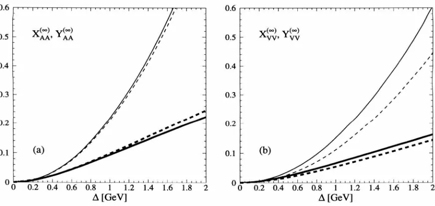
3.4 X(00)(~) and y(oo)(~) for the a) axial, and b) vector coefficients. Thick

solid lines are X while thick dashed lines are Y. The thin solid and dashed lines are X and Y to order ~2 _/m~

b· '

4.1 (a) The relevant term in the operator product expansion. Wavy lines

denote the insertions of left-handed currents. (b) does not contribute 33

34

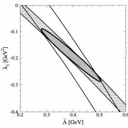
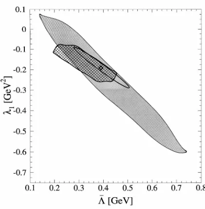
to b ---+ c decay. . . . . . . . . . . . . . . . . . . . . . . . . 41 4.2 Allowed regions in the

A->.

1 plane for R1 and R2 with 1/m~ corrections

omitted. The bands represent the lO" statistical errors, while the ellipse

4.3 Extraction of

A, ,\1 .

Cross and ellipse show the values of

A, ,\1

ex-tracted without 1/m~ corrections but including the experimental sta-tistical error. Shaded region: Higher order matrix elements estimated by dimensional analysis. Cross-hatched region: p1 = 0.13GeV3, p2 = 0. 56

List of Tables

2.1 Observed heavy mesons and their assignment to HQS doublets.

5.1 Central values of 8m1(xa) and 8m2(xa) for two different values of ms.

r

=

4 · 10-4 _{corresponds to ms}

=

_{100 MeV, while r}

=

_{1 · 10-}2

corre-sponds to a constituent quark mass ms

=

500 MeV. For mb ~ 4.8 GeV,

xa

=

0.91, xa

=

0.83 and xa

=

0. 75 correspond to Ea

=

2.2 GeV, 9

Chapter

1

Introduction

"My father and mother were honest, though poor-"

"Skip all that!" cried the Bellman in haste.

"If it once becomes dark, there's no chance of a

Snark-"We have hardly a minute to waste!"

Lewis Carroll [1]

The current theory of electroweak and strong interactions (the Standard Model) has

been confirmed by numerous experiments and is now regarded as the correct theory

of particle interactions in the energy range up to about 100 GeV. Among the many

stringent tests it has passed the most spectacular ones were the precision

measure-ments of various observables at LEP, where the predictions of the Standard Model

were tested with accuracy of fractions of a percent. In modern parlance, this success is expressed by saying that the low-energy effective Lagrangian (for energies below

100 Ge V) is indeed the Lagrangian of the Standard Model. There are reasons to

be-lieve that at higher energies new particles and interactions come into play, but their

effect on low-energy physics can always be accounted for by adding local operators of

dimension higher than four to the Lagrangian. Therefore such effects are suppressed

by powers of the scale of new physics.

But knowing the Lagrangian is not the same as being able to make quantitative

predictions for physical observables. The dynamics of the Standard Model is so

com-plicated that not even all its qualitative features are understood (e.g., confinement of

color.) The problem is that strong interactions become so strong at low energies that

fundamental constituents, quarks and gluons, are permanently bound inside hadrons

(mesons and baryons). Understanding the properties of hadrons is highly nontrivial,

since it requires techniques beyond perturbation theory. (The only available

about twenty years old.) This is why theoretical particle physics became an art of

finding physical quantities which can be both accurately predicted and at least m

principle measured.

Unlike other high arts, however, this art needs a raison d'etre. One motivation

is to be able to confront the Standard Model with experiment and hopefully

un-cover a more fundamental theory underlying it. For example, the aforementioned

confirmation of the Standard Model predictions at LEP has become possible only

because it was realized that at high energies the strong interactions become weaker

(this is the asymptotic freedom of strong interactions discovered by Gross, Wilczek,

and Politzer [2].) Another motivation is the desire to measure the parameters of the

Standard Model Lagrangian as accurately as possible. There are about twenty such

parameters (quark and lepton Yukawa couplings, gauge couplings, etc.), and a more

fundamental theory must be able to predict some of them.

It was realized quite some time ago that hadrons containing heavy quarks, band

c, 1 _{are more tractable than the light ones. The reason is twofold: first, under}

fa-vorable circumstances the large energy scale involved enables one to argue that, by

virtue of asymptotic freedom, the perturbative calculation provides a reasonable first

approximation. Second, new approximate symmetries arise in the limit of large quark

masses, resulting in many new relations between physical quantities. Using these

ob-servations, a lot of progress in our understanding of hadrons containing a single heavy

quark has been made in the last few years. One consequence of these theoretical

de-velopments was a better measurement of several Standard Model parameters, notably

the heavy quark masses, and the Cabibbo-Kobayashi-Maskawa angles l°Vc:bl and, to

a lesser extent,

IVubl·

This work describes some of this progress, focussing on the

precision measurements of the abovementioned parameters. After introducing the

necessary theoretical background in Chapter 2, we discuss in Chapter 3 the

model-independent determination of

I

°Vc:b

I

in the exclusive semileptonic decay B ---+ D* f D.

Chapter 4 is devoted to the inclusive B decays and their use in the measurement of

l°Vc:bl, the heavy quark masses, and certain nonperturbative matrix elements

terizing the structure of the heavy mesons. In Chapter 5 we describe how the rare

decay b--+ S/ can be used to measure precisely the bottom quark mass. Concluding

Chapter

2

Theoretical background

2.1

Heavy qua

r

k symmetry

"You boil it in sawdust: you salt it in glue:

You condense it with locusts and tape:

Still keeping one principle object in view

-To preserve its symmetrical shape."

Lewis Carroll [1]

Consider a hadron containing a quark with a mass mQ much bigger than the

characteristic scale of strong interactions, AQCD· It is clear that the energy and mo

-mentum of the light constituents (gluons and light quarks) will be of order AQcD,

and the velocity of the heavy quark in the rest frame of the meson will be of order

\

v\ ,...,

AgcD ~ 1. This means that in the first approximation the heavy quark can

fflQ

be treated as a static source of the chromoelectric field. Further, since the

chromo-magnetic moment of a quark is inversely proportional to its mass, the heavy quark

spin decouples. We conclude that the light constituents of the hadron (collectively

known as the "brown muck") are sensitive to neither the mass of the quark (provided

it is big enough for the static approximation to be applicable), nor the orientation of

its spin. In general, when properties of a physical object are not changed by certain

kinds of tampering, physicists call these allowed kinds of tampering symmetry

trans-formations. If we have N flavors of heavy quarks, each of spin 1/2, we can substitute

one flavor of quark for another, or flip the spin of the quark, without changing the

structure of the "brown muck." This approximate symmetry is called Heavy Quark

Symmetry (HQS) [3], and the corresponding transformations form a unitary group

U(2N). In the real world, only band c quarks deserve to be called heavy, so HQS will

HQS is not manifest in the QCD Lagrangian, which makes it a bit hard to use

(see however Ref. [3]). To make it explicit, one has to pass to an effective field theory

description of strong interactions, with all short-wavelength fluctuations capable of

noticing the tampering integrated out. If we limit ourselves to systems containing

one or zero heavy quarks at a time, the number of heavy quarks of each flavor in

this effective theory is conserved, since producing heavy pairs requires hard quanta

in the initial state. In such a theory the relation between a heavy quark Q and its

antiparticle

Q

is lost, and each of them is described by a separate field. In fact, since

we will be dealing exclusively with systems containing just one of them, say Q, we may forget about the

Q's

from now on. The Q's will then be described in our theory

by a spinor field h(x) with two independent components.

By now it should be clear that what we are trying to do is very similar to the

stan-dard Foldy-Wouthuysen transformation. In fact, at tree level (if we treat the color

field as the classical background) it is exactly the Foldy-Wouthuysen transformation.

At this level the relation between the full quark field Q(

x)

and its effective theory

rela-tive h(x) is given by well-known QED formulae [4], with electromagnetic potential and field strength replaced by their QCD counterparts. Of course the Foldy-Wouthuysen

procedure breaks Lorentz invariance of the theory, but this is to be expected: after all

there is a preferred frame in this problem, the rest frame of the heavy meson. Still,

it is convenient to preserve at least Lorentz covariance by letting the preferred rest

frame have an arbitrary 4-velocity v. Then the heavy quark will be described by a

v-dependent Dirac spinor hv ( x) satisfying

l+p

-2- hv(x)

=

hv(x). (2.1)

This constraint ensures that the field hv ( x) has only two independent components,

which describe the two spin states of the heavy quark. In the rest frame of the meson,

where v = (1, 0), Eq. (2.1) reduces to the requirement that the two lower components

of hv be zero. "Covariantizing" the standard formulae from Ref. [4], we arrive at the

where Dµ

=

8µ - igAµ is the covariant derivative, and D l..

=

D - v( v ·

D).

Similarly,

we can easily read off the tree level Lagrangian for hv from Ref. [4]:

£

(2.3)

Beyond tree level, the Lagrangian of the Heavy Quark Effective Theory (HQET)

must be constructed as the most general linear combination of local operators built

out of hv(x) and other fields which is consistent with the symmetries of QCD. The

coefficients in this Lagrangian are determined by matching amplitudes in HQET and

full QCD order by order in a5 • The higher the dimension of the operator, the more

its coefficient is suppressed by powers of mQ. Therefore only a few operators will be

relevant in practice. Actually, there is an ambiguity in this construction related to

the freedom to redefine the heavy field hv ( x). To eliminate this ambiguity, we will

require that hv( x) and h! ( x) have canonical commutation relations.1 This ensures

that at tree level the part of the effective Lagrangian depending on hv is identical to

the Lagrangian obtained by the Foldy-Wouthuysen procedure, Eq. (2.3). The leading

(dimension-four) contribution to the HQET Lagrangian has the following form [5]:

LHQET = hv iv· Dhv

+

L/ight1 (2.4)

where L/ight is the standard QCD Lagrangian for gluons and light quarks. (One

could think that there is a candidate operator of dimension three as well, namely

hvhv. However its coefficient can always be made zero by redefining the heavy field

according to hv(x) --t eiav·xhv(x) with some a.) Since we required that hv and h!

were canonically conjugate variables, higher-dimensional contributions to the HQET

Lagrangian will not contain the "time derivative" v · D acting on hv.

The Lagrangian Eq. (2.4) has manifest HQS: it does not care about either spin or

flavor of the heavy quark. Higher dimensional contributions will break this symmetry.

The corrections due to operators of dimension five are

Ckin h- (

·n

)

2 _h

+

_Cmag

li

_{!]_ Ql-L" h}

2 ffiQ v i .l. v 2 ffiQ v 2 ()' µ11 v.

(2.5)

In Eq. (2.5) only the operators which depend on hv(x) are included.2

The coefficients in Eq. (2.5) are determined by matching amplitudes in HQET and

full QCD order by order in perturbation theory. Thus we are making a double

expan-sion in 0'.5 and 1 / mQ. Beyond tree level matching requires choosing a renormalization

scheme. Physically, the most transparent renormalization procedure would be to cut

off the loop integrals in HQET at some scale A. This is the Wilsonian renormalization

group approach. Technically, it is much more convenient to use dimensional

regular-ization and the MS subtraction scheme both for HQET and full QCD diagrams, with

the subtraction point µ replacing the ultraviolet cutoff A. This is what we are going

to do in what follows.3

Both Ckin and Cmag are 1 at the tree level. It can be shown that Ckin = 1 to all

orders in 0'.5 [6]. The coefficient Cmag has been computed to order a5 , and leading

logarithms of the form a~ logn ~ have been summed up [7]. The result is

C ( ) =

(

as(mQ)

)

3

/

fJ

o

(i

13 0'.5 )

mag µ ( )

+

6 ,

O'.s µ 7r

(2.6)

where (30

=

11 - 2n1 /3.

The contribution from dimension-six operators being suppressed by extra power

2_{To be precise, we must specify what mq means. For us, mq will always denote the quark pole}

mass.

3_{The admissibility of dimensional regularization in HQET was a subject of some debate. Our}

of mQ relative to Eq. (2.5), we will need it only at the tree level. The corresponding

expression can be read off Eq. (2.3):

(2. 7)

+

Although Eq. (2.7) seems to contain the time derivatives of hv, it can be rewritten in

a form in which only spatial derivatives show up. This is a consequence of how the

Foldy-Wouthuysen transformation is constructed.

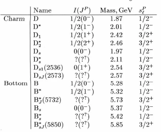
Let us apply this formalism to the spectroscopy of heavy mesons. By virtue of HQS, the spin of the heavy quark is conserved, and therefore the total angular momentum of the "brown muck" is conserved too. Thus we can label the heavy

meson states by their parity P, total spin j, and the spin of the light degrees of freedom Sf.. The heavy quark spin being 1/2, for fixed St the total spin can take

values j = St ± ~- HQS implies that these two states are degenerate. Thus heavy

mesons come in doublets labeled by

sf.

This is what is observed in nature - see

Table 2.1.4 _{HQS also predicts that the splitting between the ~ - and ~+ doublets}

is the same for charmed and bottom mesons. This also seems to be true, if all the resonances with undetermined quantum numbers are interpreted as what their names

suggest.

To understand the deviations from the HQS predictions, let us derive the meson

mass formulae to order A~

0

0

/m~ [9, 10, 11]. (We will use these formulae extensively

in the following chapters.)

First let us introduce some notation. Let

I

H ( v)) be the state representing a heavy meson with 4-velocity v

=

(1,

0).

It is an eigenstate of the full QCD Hamiltonian with the eigenvalue mH. Let 1iHQET be the Hamiltonian corresponding to the Lagrangian

Eq. (2.4), and 1t

=

1iHQET +/::).}{,be the Hamiltonian derived from the Lagrangian

LHQET

+

6.£, where 6.£

=

6.£5

+

6.£6

+

..

.

represents corrections from operators of

Name J(JP) Mass,GeV Sp

e

Charm D 1/2(0-) 1.87 1;2

-D* 1/2(1-) 2.01 1;2-D1 1/2(1+) 2.42 3/2+

D* ₂ 1/2(2+) 2.46 3/2+ Ds

O(o-)

1.97 1;2-D* _s

?(?7)

2.11 1;2-Ds1 (2536) 0(1 +) 2.54 3/2+

DsJ(2573)

?(??)

2.57 3/2+ Bottom B 1/2(0- ) 5.28 i;2

-B* 1/2(1-) 5.32 1;2-Bj(5732)

?(?7)

5.73 3/2+ Bs

O(o-)

5.37 1;2-B* _s

?(??)

5.42 1;2-B;J(5850)

?(?7)

5.85 3/2+

Table 2.1: Observed heavy mesons and their assignment to HQS doublets.

dimenision five and higher. By construction, 6,.£ does not contain time derivatives,

therefore 6,.1{ =

-6,.

£

.

The effective theory Hamiltonian 1{ being equivalent to the

full QCD Hamiltonian, [

H(v))

is an eigenstate of

H

.

The corresponding eigenvalue

is mH - mQ, since in the effective theory the energy is counted from the rest mass

of the heavy quark. Finally let us denote by [ H00(v)) the limit of [

H(v))

as mQ---+

oo. Evidently, this limit exists and is the eigenstate of 'HHQET· We denote the

corresponding eigenvalue by

A.

Our starting point is the identity

[

1 (H

oo

(v)

IHI

H(v))

l

mH = mQ

+

2

(Hoo(v)

I

H(v))

+

h.c

.

.

(2.8)

Using the definitions of 1{ and

I

H00(v)), and the Gell-Mann and Low theorem (see, [image:16.543.63.330.42.262.2]

Expanding Eq. (2.9) up to terms of relative order 1/m~ we obtain the mass formula:

mH

mQ

+A -

(H

oo

(v)

l.6.£s

+

.6.£6\

H

00

(v))

(2.10)

- [

~(H

oo

(v)

l.6.£s(O) i

j

d

3x

j_

0

00

dt

.6.£s(x)I

H

00(v))

+

h

.

c.

]

.

.6.£s and .6.£6 are given by Eq. (2.5) and Eq. (2.7) respectively. We normalize

one-particle states to 1 per unit volume here and in what follows.

Eq. (2.10) contains expectation values of both local and nonlocal operators. When H is the ground-state

(sf

= ~ -) doublet, it is convenient to introduce a shorthand notation for these expectaion values:

(H

oo

(v)

\

hv (iD.L)

2

hv I

H

00

(v)),

d~

(H

oo

(v)

I

hv

~

CYµv cµv hv

I

H

oo

(v))'

(H

oo

(v)lhv(iD

01

)(iDµ)(iD

f3

)hv\H

00

(v))

=~PI

(g01

{3

-

V

01

V

{3

)

Vµ,

(H

oo

(v)

\

hv(iD

Ol

)(iDµ)(iDf3) /8/s hv

\

H

00

(v))

= ~dHP2

it

v01f3o

Vvvµ,

(2.11)

(2.12)

(H ( _oo

v

)

1

-h ('

v

zD.L

)2

h

v

z

·

j

d

3

x

J

O

_{dt.6.£s(x)IH}

Ti+dHTi (

)

00(v))

+

h.c.

= , 2.13

-oo

mQ

(H

oo

(v)\h

v

!]_

CYµv

cµv

hvi

J

d

3_x

1

°

dt.6.£s(x)

I

H

oo

(v))

+

h

.

c.

=

73

+

dHTt'

2 -oo

mQ

where

dH

=

3 or -1 depending on whether

H

00 is a pseudoscalar or a vector. In

terms of these matrix elements the meson mass is given by

(2.14)

In particular, the leading order deviations from HQS are described just by two matrix

elements of local dimension-five operators, ,\1 and A2. Dimensional analysis suggests

by the same two matrix elements, so it is important to know their numerical values.

According to Eq. (2.14),

Cmag(µ)>.. 2(µ)

determines the splitting between the

mem-bers of the ground-state doublet. Therefore, if one neglects the corrections of order

Atco/mL one can use the measured splitting between Band B* mesons to extract the

value

Cma

9

(µ)>..2(µ)

'.::::::'.

0.12GeV

2

.5 It is much harder to determine _{>.. 1}. In Chapter 4

we show how one can extract )..1 and

A

from the measured charged lepton spectrum

in the inclusive semileptonic B decay.

In the following chapters we will often need the values of the quark masses mb

and me to make numerical estimates. According to Eq. (2.14) the difference mb - me

is given by

mb - m = _ mB - mD -_ _{>.. 1} ( 1 - - - - -1 )

+

0 ( Aqco

3

)

e 2mD 2mB

m'IJ

'

(2.15)

where mB

=

(mB

+

3mB• )/4, mD

=

(mD

+

3mD• )/4. QCD sum rule estimates of >..1

range from -0.1 GeV2 to -0.6 GeV2 [13, 14]. Roughly the same range results from the

analysis of Chapter 4. Thus we take )..1 = -0.3±0.3 GeV2. As for the error from terms

of order Aqco3 /m'YJ, we conservatively estimate it as (0.5GeV)3

/m'b '.::::::'.

0.03 GeV.

Then Eq. (2.15) implies mb - me

=

3.39 ± 0.08 GeV. To determine mb and me

separately, one needs to know

A.

QCD sum rules give

A

= 0.5 ± 0.1 GeV [13]. This value for

A

is consistent with the results of Chapter 4, although the latter have much

larger uncertainty. According to Eq. (2.14) mB = mb

+A+

O(Aqco2 /mb), so using

A

=

0.5 ± 0.1 GeV we obtain mb

=

4.8 ± 0.1 GeV. On the other hand, estimates

of mb based on sum rules for bottomonium give contradicting results [15], but in

general produce values in the range 4.55 - 4.8 GeV. To be conservative, we adopt

mb

=

4.8 ± 0.2 GeV. Then me

=

1.41 ± 0.28 GeV.

We would like to conclude this section with a lightning review of the use of HQET

m the study of exclusive weak decays. HQET is particularly useful when applied

to semileptonic and radiative decays of heavy hadrons. Here one must distinguish

between heavy-to-light and heavy-to-heavy decays. HQS relates various amplitudes

5_Both

in each class. For example, it relates the form factors describing D ---+ p and D ---+ ]{* transitions to those describing E ---+ p and E ---+ ]{* transitions respectively. This

can be used, in principle, to accurately measure

I

Vub

l

[16]. Here we will focus on heavy-to-heavy decays. Since in real life the only heavy quarks are b and c quarks, we will sacrifice "generality" to the transparency of notation, and discuss the matrix elements of flavor-changing b-to-c currents between EH and D(*). This is a partic-ularly interesting situation, since EH and DH belong to the same HQS multiplet.

Consider the matrix element

(2.16)

where Jr= cf b, and

r

is either/µ or /µ/5 . The differential rate of the semileptonic

decay E(*) ---+ D(*}.f,;; can be expressed through these matrix elements. The first step

is to find the HQET operator corresponding to the full theory operator Jr. This

"matching" should be done order by order in perturbation theory. At tree level, we can use Eq. (2.2) to express the heavy quark fields

c(

x) and b( x) in terms of the

HQET fields h~(x) and h~(x). Then the operator Jr becomes

(2.17)

Beyond tree level, one should allow for all possible operators with the correct

quan-tum numbers to appear on the right-hand-side of Eq. (2.17). Their coefficients are

determined by the requirement that the matrix elements of the current in the full theory and in the effective theory agree to all orders in as and 1/mc,b· For example,

neglecting all corrections of order 1 / mc,b, one expects to find for the vector and axial currents

3

Jv '"""'c(i)( I ) h-c r hb

L...J V V · V ' µ v' i v' (2.18) i=l

3

JA '"""'c(i)( I ) -he r hb

L...J A V • V , µ v' i /5 v,

where

(2.19)

The peculiarity of HQET is that the matching coefficients C(i) depend on v · v'.

Because of this, even the one-loop expressions are fairly complicated [17).

Neglecting the 1/mQ corrections both to the currents and to the meson states,

and keeping in mind Eqs. (2.18), we are led to consider

(2.20)

Here IDtl) and IBt l) are the states in the infinite mass limit, and therefore are just

tensor products of the heavy quark spin state and the "brown muck" state. Noticing

that the current acts only on the heavy quark degrees of freedom, we infer that the

matrix element Eq. (2.20) is given by

-e(v ·

v',µ) Tr[M(v')r M(v)],

(2.21)

where

e(

v · v'

,

µ)

is a universal form factor, and

M( v)

is the projector on the

appropri-ate stappropri-ate of the HQS doublet. Using the nonrelativistic normalization of stappropri-ates (one

particle per unit volume), these projectors can be computed to be

1

+

p

{

-1s for the pseudoscalar

M(v)

=

m

.

2v 2

¢

for the vector

(2.22)

Thus, if one neglects the 1/mQ corrections, all the form factors are expressed through

a single function

e,

known as the Isgur- Wise function.

The Isgur-Wise function cannot be computed perturbatively. However, its value

at zero recoil ( v · v' = 1) is fixed by HQS to be 1. To see this, consider the matrix

element of the flavor-conserving current h~/µh~ between the B-meson states

IE=

)

with the same velocity. By HQS, it is given by Eq. (2.21) with v

=

v'. A short

computation shows that the matrix element in question is just given by

e(1 )vw

On

eigenstate of the corresponding charge with eigenvalue l. This proves that ~(1)

=

l. In the next chapter we will see how this fact can be used to accurately measure

I

Vcb

I

in the exclusive decay B ---+ D* Rv.

2.2

Heavy quark expansion

Since the mid seventies, inclusive weak decays of heavy hadrons were described using

the parton model. In other words, in order to predict the rate and the spectrum of

final states in a certain inclusive decay, one just computed the coresponding quantities

for the free heavy quark decay. The justification for such a procedure was that these

decays occur on a short time scale, the energy release being large. Therefore one

could argue that the total probability for a heavy quark to decay does not depend

on the "brown muck." The situation with final state spectra was less clear, but it

was known that the lepton spectrum in the inclusive B and D decays agrees with

the parton model predictions quite well. An ad hoc model of Altarelli

et

al., [18]

which attempted to incorporate the effect of the heavy quark "Fermi motion," led to the same conclusion. However, the limits of the parton model description remained unclear. Only relatively recently was it realized [19] that in many cases one can justify

the parton model, and even compute corrections to its predictions, using the Operator

Product Expansion (OPE) and some additional qualitative assumptions collectively

known as quark-hadron duality.

The basic idea of Ref. [19] is simple enough. Suppose we are interested in an inclusive weak decay of a heavy hadron H which is mediated by a quark bilinear

Jr =

qr

Q. Here Q is the initial heavy quark, and q is the final state quark which

may or may not be heavy. Consider the expectation value of the time-ordered product

T(q

2

,q · v)

= -i

j

d

4

xe-iq·x(H(v)IT

[J/(x)Jr(O)]

IH(v)). (2.23)

c

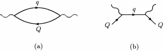
Figure 2.1: The analytic structure of the time-ordered product of two heavy quark currents.

this need not concern us here. Let us also define

W(q2, q ·

v)

= (27r)3

L

84 (PH - q - PX) (H(v)IJtlX)(XIJIH(v)). (2.24) x

The differential decay rate can be expressed in terms of W. It is easy to see that

W = -~ImT. It is convenient to regard T as a function of complex variables q2

and q · v. The analytic structure of T at fixed real q2 _{in general looks like Fig. 2.1.} The two cuts correspond to two possible time orderings of the currents in Eq. (2.23).

Only the ordering giving the left cut corresponds to the decay process, the other cut

corresponding to the states containing two Q's. W may be regarded as a discontinuity

of T across the physical cut.

Of course, computing T for all q2 and q · v is beyond our capabilities. However,

far away from the cuts T can be computed using the OPE, since in this situation all

intermediate states are highly virtual. More concretely, the time-ordered product of

currents always admits a short distance expansion of the form

T [lt(x)Jr(O)]

x~o

L

Co(x)O(O),

(2.25) [image:22.536.183.386.58.245.2]

16

where 0 are local operators, and Co are c-number coefficients. If q is chosen so

that all physical intermediate states are far off-shell, then we expect that the Fourier

transform of Eq. (2.25) will be dominated by several operators of lowest dimension,

whose coefficients can be computed in perturbation theory.

How can we use our knowledge of T in the unphysical region of the q · v plane?

Suppose we would like to compute the inclusive differential rate dI' / dq2. It is given by

an integral of W with an appropriate weight along the physical cut. The lower limit

of the integral depends of the nature of the process, but the upper limit is always the

end of the physical cut. This integral can be interpreted as an integral of T along

the contour shown in Fig. 2.1. The integrand can be computed everywhere on the

contour except where it touches the cut. Neglecting this problem for the time being,

we may conclude that df / dq2 is calculable by means of the OPE. Similarly, one can

argue that other inclusive observables are calculable.

The problem is simplified further by the observation that one may keep track only

of those operators whose expectation values in the initial hadron state are nonzero,

and only if the Fourier transform of their coefficients has a discontinuity across the

cut in the physical region. For example, at leading order in a8 , the coefficient of

the unit operator is given by the diagram in Fig. 2a, while the the coefficients of all

operators of the form

Qr

A

Q

can be extracted from the diagram in Fig. 2b. But it is

easy to see that the diagram in Fig. 2a has no imaginary part for values of q relevant

for the decay process in question, and therefore the unit operator may be omitted.

Typically, the relevant operators are of the form QDµ1 • • • DµnQ (we omitted the

Dirac structure). To argue that only a few operators of lowest dimension are

im-portant, one has to show that derivatives scale like AQCD· In fact, this statement is

just plain wrong if

Q

is the ordinary quark field, since the time-like component of

the heavy quark momentum is very nearly mQ. However, it is rather obvious how to

circumvent this problem: one has to perform the OPE in terms of the "rescaled" field

QeJJ(x) = eimQv·xQ(x) rather than in terms of Q(x). Then the derivatives will bring

q

Q

(a)

(b)

Figure 2.2: Diagrams representing the OPE coefficients at the tree level. The co-efficient of the unit operator is given by diagram (a). The coco-efficients of the heavy quark bilinears

Qr

AQ can be determined from diagram (b). Wavy lines denote the insertions of the current if.

r

Q.

mQV subtracted, which is indeed of order AQcn.6 Recall that the relation between

Q(x) and the HQET field, Eq. (2.2), involved the same factor eimqv·x. Thus it is

natural (though not absolutely necessary) to go one step further and to do the OPE

in terms of the HQET field hv(x). The advantage is threefold. First, hv(x) satisfies

the constraint Eq. (2.1), which makes the Dirac algebra simpler. Second, counting

powers of mQ is more straightforward in HQET than in full QCD. Third, the number

of nonperturbative matrix elements parametrizing the decay rate can be reduced by

taking into account the requirements of HQS. In the effective theory this is very easy

to do, since HQS is manifest.

For example, for semileptonic B-decay the leading (dimension three) operator in

the OPE is Q1µQ, the conserved current, and its expectation value is just Vµ- It

is not necessary to pass to the effective theory to evaluate it. The contribution of

this operator to the differential decay rate is exactly the parton model result. The

only dimension four operator is hvDµhv. Using the equations of motion of HQET,

its expectation value in the B-meson state can be expressed in terms of the

expec-tation values of dimension five operators [20]. Because of this, the corrections to the

parton model result are suppressed by two powers of mQ. They are parametrized

by the matrix elements of two dimension five operators: the kinetic energy operator

hv( iD

1.)

2 _{hv, and the chromomagnetic operator hvO" · Ghv. Their expectation values}

are just .\1 and .\2 defined in Eq. (2.11).

[image:24.540.133.416.62.152.2]

Naturally, there are limitations to this approach. The OPE works only if the

intermediate states are far off-shell. For this to hold everywhere on the contour in

Fig. 2.1, the distance between the cuts must be of order 1 Ge V or more. In b --+ c

decays the cuts are always separated by at least 2mc, and over most of the phase

space the distance is of order mb. These are large enough scales for the OPE to be

applicable. On the other hand, in b --+ u decays the cuts merge when q2 is maximal,

i.e., when the leptons are back-to-back. Thus the OPE fails in one corner of the Dalitz

plot.

It remains to discuss what to do with the parts of the contour in Fig. 2.1 which lie

near the cut. Here the notion of quark-hadron duality [21] comes in handy. Notice that

the expression for T as given by the OPE has analytic structure similar to Fig. 2.1,

except that the positions of the cuts are determined by the heavy quark mass mQ

rather than by the hadron mass mH. One can think of the OPE as computing the

decay rate in terms of quark and gluon degrees of freedom, although the actual final

state consists of hadrons. In fact, the leading term in the OPE is always the same

as the parton model result. Of course, we cannot expect the parton model to exactly

reproduce W, since the latter may receive contributions from hadronic resonances

which are absent in perturbation theory. However, if the hadronic invariant mass is

large, the resonances must be very broad and overlap significantly. In this case we

do expect perturbation theory to reproduce W accurately. This is the postulate of

local quark-hadron duality [21]. It seems very reasonable from the physical point

of view and has numerous experimental confirmations, e.g., in e+e- annihilation. A

less stringent assumption is that the OPE reproduces W smeared over an interval of

hadronic masses of order AQCD· We will refer to this as global quark-hadron duality.

The upshot of the above discussion is that if the contour approaches the cut where

the hadronic invariant mass is allowed to be large, we can justify using the expression

for T obtained from the OPE. This is the situation for the total semileptonic decay

rate B --+ Xcf D. Moreover, the above argument shows that the lepton spectrum

is also computable using the OPE provided we do not come too close to the end

is close to the maximum. Similarly, global quark-hadron duality tells us that we can

compute the properties of the averaged hadron spectrum. If we were bold enough to

trust local duality, we could also compute the hadron spectrum point by point for the

region where the hadronic mass is large.

In principle, the ability to predict the inclusive semileptonic B width enables one

to measure precisely the mixing angle

IVcbl·

The difficulty is that the prediction also

contains the quark pole masses mb and me which are not well known. The mass

formulae of Section 2.1 can be used to express mb and me in terms of well known

meson masses and various nonperturbative matrix elements. If we neglect

dimension-six operators, we are left with only with three of them:

A, .\

1 and .\2 . As mentioned

previously, the value of .\2 is known, while the values of the other two are not. One

possibility is to try to determine

A

and .\1 using QCD sum rules [13, 14). Another

is based on the observation that these same two quantities influence the shape of

the lepton spectrum in the decay B --+ Xefil, and therefore can be extracted from

experiment. This possibility is explored in Chapter 4. Still another way to measure

A

and .\1 (in the decay B--+ Xs1) is discussed in Chapter 5.

2.3

Renormalons as a red herring

To compute OPE coefficients beyond tree level one has to choose a regularization

procedure. Usually, dimensional regularization is the most convenient method because

it maintains gauge invariance and automatically subtracts power divergences. But

often it is argued that, unlike a sharp momentum cutoff, dimensional regularization

does not achieve the strict separation of scales. If this were true, one would be forced

to abandon dimensional regularization, since separation of short- and long-distance

physics is the very idea of the OPE. However, the abovementioned arguments are not

entirely convincing.

At any finite order of perturbation theory there does not seem to be a problem.

scale Q:

(2.26)

Here Ci are perturbatively calculable coefficients, and Oi are operators of dimension

i. One could regard Eq. (2.26) as a way to present A( Q) so that the power-like

dependence on

Q

is made explicit. The logarithmic dependence is buried in Ci and

Oi. The coefficients Ci can be computed in perturbation theory, while for matrix

elements (

oi)

only the

Q

dependence can be determined.

The difficulties start when one tries to give the expansion in Eq. (2.26) a

mean-ing beyond perturbation theory. Apriori, it is not clear that the series definmean-ing the

coefficients C; are convergent. In fact, there are reasons to believe that they are only

asymptotic [22]. One popular approach to this problem is to define the sum of an

asymptotic series using the Borel prescription. Let us consider a series

(2.27)

The idea behind the Borel prescription is to consider an associated series

S ( )

B

t

= ai

+

a2

t

+

- t ...

a3 2

+ -

an+ ₁- t 1 n

+ ...

2 n. (2.28)

Suppose this new series converges and defines an analytic function for all nonnegative

t.

Then the sum of the series Eq. (2.27) is naturally defined as

(2.29)

It is easy to check that the expansion of the integral Eq. (2.29) in powers of x

repro-duces Eq. (2.27). The problem arises if SB(t) has poles on the positive real axis. Then

the integral in Eq. (2.29) is not well-defined, and the Borel prescription is ambiguous.

These ambiguities are called renormalons.

It is often said that if the OPE has a meaning beyond perturbation theory, then the

would prefer to have converging series, but, lacking convergence, Borel-summability

is argued to be the next best thing. Our first objection is that Borel prescription

is ad hoc: there are other ways to define a sum for an asymptotic series (see, e.g.,

Ref. [23]). Further, it is stated that dimensional regularization yields series which

contain renormalons, and therefore is deficient. Let us inspect this argument more

closely. It is extremely difficult to establish the large-order behaviour of perturbation theory. No rigorous results (even at a physical level of rigour) have been obtained for

D

=

4 field theories. Instead, the argument is based on the large-order behaviour of

a small gauge-invariant subclass of Feynman diagrams. They are obtained from the

tree diagrams by insertion of a chain of one-loop vacuum polarization diagrams into

the gluon propagators. Technically, the summation of these contributions amounts to

replacing 0'.8 (µ) by 0'.8 ( k), where k is the momentum flowing through the propagator.

Since

as(k)

has a pole at

k

=

AQco, the result is ambiguous. This is how renormalon

ambiguity manifests itself here. Therefore, the argument goes, the dimensionally

regularized Ci pick up unwanted and ambiguous infrared contributions which in all

honesty should reside in

(Oi)·

In other words, there are ambiguities in both Ci and

( Oi),

and only their product is well defined. However, if one imposes a sharp infrared

cutoff at k

=

b.

>

AQco, the result is well defined, and there are no renormalons

in Ci. An obvious flaw in such reasoning is that it relies on the summation of a

small subclass of diagrams. This subclass does not dominate in any reasonable limit

of QCD, and thus the actual behaviour of the perturbation theory may be quite

different. In particular, there is no guarantee that imposing a sharp cutoff makes the

series Borel summable.

From the practical point of view, the issue of renormalons is irrelevant. After all,

we can compute only a couple of terms in perturbation theory, and what happens

at large orders is of purely academic interest. The relevant question is what is the

meaning of the matrix elements

(Oi)

in the absence of a nonperturbative definition

of the OPE. The answer is that one should regard them as uncalculable parameters

which must be determined by fitting Eq. (2.26) to experimental data. Once the

be worried that since the coefficients C; are known only to a finite order in

as(

Q),

neglecting higher orders in perturbation theory may introduce large uncertainties

in the extracted values of the "condensates" (O;). Indeed, at sufficiently large

Q

the neglected terms in C0 are always larger than the condensate contributions, since

the former are suppressed by powers of log Q2 _{while the latter are suppressed by}

at least Q2

• The resolution is that the extraction of condensates by fitting A( Q)

is possible only if there is a range of Q in which the neglected terms in Co are

small, while the condensate contribution is still important. The existence of such a

range can be settled only on a case-by-case basis [24]. Similarly, the measured values

of the condensates can be used to improve predictions for other observables only

if the the neglected perturbative corrections are small compared to the condensate

contributions. Otherwise perturbative uncertainties dominate, and one gains nothing

by including nonperturbative effects.

Similar issues are involved when one tries to extract (O;) from lattice Monte-Carlo

simulations. In fact, one may regard such simulations as some kind of "experiment,"

Chapter 3

The decay

B

- 7

D*fJJ

and the

precision measurement of

IV

cb

l

3.1

Model-independent predictions for the

B

~

D*

f

v

rate at zero recoil

"The result we proceed to divide, as you see,

By Nine Hundred and Ninety and Two;

Then subtract Seventeen, and the answer must be

Exactly and perfectly true."

Lewis Carroll [1]

Hadrons containing one b quark decay mainly into charmed hadrons. Other decay

modes (Cabibbo suppressed b - u transitions, B - J/'lj;X decays, etc.) constitute

only about 1

%

of the total decay rate. Among the b - c decay modes the exclusive

decay B - D*fi/ is particularly interesting because it offers a possibility to accurately

measure the Cabibbo-Kobayashi-Maskawa angle

I

Y'c:b

l·

The reason is that HQET

makes definite predictions for the form factors describing this transition at zero recoil,

i.e., when the final state D* meson has zero velocity in the rest frame of the the initial

B meson. In this section we review how the HQET predictions arise. The next section

is devoted to the so called zero recoil sum rules. These sum rules, first obtained in

Ref. [9] and further investigated in Refs. [25, 26], can be used to estimate the accuracy

The form factors for the semileptonic B ---+ D(*)fv decay are defined as 1

2 (D(v')IVµIB(v))

2 (D*(v',

c)IVµIB(v))

2 (D*(v',

c)IAµIB(v))

h+(w)(v

+

v')µ

+

h_(w)(v - v')µ,

hA₁ (w)(w

+

l)c*µ -

hA2(w)(c* · v)vµ

hA₃(w)(c* · v)v'µ. (3.1)

Here Vµ = c1µb and Aµ = C/µ/sb are the vector and axial vector currents. (The axial

form factor between B and D mesons vanishes identically because of requirements of

parity and Lorentz invariance.) The four-velocities of the initial and final states are

denoted by v and v' respectively, and w = v · v'. The polarization vector of the D*

meson is denoted by c.

The part of the effective weak Lagrangian relevant for semileptonic b --t c decays

reads

(3.2)

where GF is the Fermi constant. The quark currents V and A have zero anomalous

dimension, and therefore the normalization point µ need not be specified.

Given the effective Lagrangian, Eq. (3.2), and the definitions in Eqs. (3.1), one

easily finds the differential decay rates:

df(B ---+ D*Rve) dw

df(B --t DRve)

dw

x

(3.3)

where r<*) = mvc-l/mB. The functions FB-.D• and FB-.D are given in terms of the

1_{The funny factors of 2 arise because we use the nonrelativistic normalization of states} (p'lp) =

form factors:

[

4w 1 - 2wr*

+

r*

2]-l

l +

-w

+

1 (1 - r*)2

x _{ 1 - 2wr*

+

r*

2

[ w - 1 ]

(1 -

r•)2

2

h~1

(w)

+

w

+

1 hi(w)

+ [

hA1 ( w)

+

~ ~ r~

( hA1 ( w) - hA3 ( w) - r* hA2 ( w))]

2

} '

1 - r

h+(w)

-1

-+-r

h_(w). (3.4)

We will be interested in the differential rate at vanishingly small recoil, i.e., for v =

v',

w

=

1. In this limit

(3.5)

According to Eqs. (2.18,2.21), if one neglects corrections of order l/mc,b, the form

factors are all expressed through a single function

e(w)

which satisfies e(1)

=

1. In

particular, the form factors h+ and _hA1 at zero recoil are given by

h+(l)

= rtv

=

cV>(l,µ)

+

c}?>(l,µ)

+

cV>(l,µ),

hA1 (1) = 'r/A ::::

C~

1

)(1, µ),

where the coefficients

C~!v

are defined in Eq. (2.18).

(3.6)

The quantities 'r/A and rtv do not depend on the renormalization scale µ. To see

why, note that for v = v' we have only one independent operator in HQET which

can match onto Aµ, namely Ji£c)/µ/sh£b). ( For v -=f v' there are three independent

operators - see Eq. (2.18).) This operator is actually one of the generators of HQS,

and therefore its matrix elements between b and c quark states do not receive any

perturbative corrections. Thus the "HQET side" of the matching calculation is

triv-ial in this case. In full theory, the operator Aµ is not conserved, but it is "partially

conserved," i.e., it would be conserved if the quark masses were zero. Partial

26

Therefore the matrix elements of Aµ, and consequently the matching coefficient 'T/A,

cannot depend on the subtraction point µ. Similarly, 'T/V must be µ-independent.

Although the matching coefficients are known only to order as, the particular

combinations entering Eq. (3.6) have been computed to order

a;

[27]. Here we write down an analytic expression for 'T/A which contains the full order as corection and part

of the order a; correction which is proportional to

/3

0

=

11 - ~n f ( n f is the number

of light quark flavors):

_ l as ( mb

+

me l me 8) a;

/3

5 ( mb + me l me 44)

'T/A - - - n -

+ -

-

-

o - n -

+

-

.

7r mb - me mb 3 7r2 24 mb - me mb 15

(3.7)

In Eq. (3. 7) as is the MS coupling evaluated at the scale yimbme. Of course, the

complete order

a;

contribution [27] contains terms which are not proportional to

/30.

Still, Eq. (3. 7) approximates the complete order

a;

result very well because

/30

is large numerically. In general, it was noticed that for many QCD observables corrections of

order

a;j3

0 provide a good approximation of the full order

a;

corrections. Examples

can be found in Ref. [28]

Putting all this together, we conclude that up to corrections suppressed by

AQco/me,b the values of IFB-+D•(l)I and IFB-+D(l)I are given by 'T/A and TJv,

re-spectively. Since measuring the differential rates df / dw near w

=

1 is equivalent to

measuring IF(l)Vcbl (see Eq. (3.3)), we can extract the value of IVcbl by studying the

decays B -+ DCv or B -+ D* Cv.

In real life me is not very large, and the corrections of order 1/me may be quite

substantial. However, Luke's theorem [29] states that for B-+ D* decay there are no corrections of order 1/me,b· There are still corrections of order 1/m~,b' and they limit

the accuracy of the extraction. The corresponding theoretical uncertainty is expected

to be of order (A/2me)2_{, where A is the characteristic scale of strong interactions.}

Setting A

=

0.5 GeV, me

=

1.4 GeV, we conclude that 1/m~ corrections to the value

of IFB-+D•(l)I are of order 3%. Therefore the theoretical uncertainty of the extraction

of \Vebl is also of order 3%. (Of course, "of order 3%" may mean 6% or even 10% in

Naturally, one would like to know better the size of 1/m~,b corrections.

Unfortu-nately, this cannot be done in a model-independent manner. In Ref. [30] the 1/m~

contribution enhanced by the logarithm log AQco/m7r has been evaluated using chiral

perturbation theory. It turned out to be negative and small, less than 0. 7% in absolute

value. Although formally this logarithmically enhanced contribution "dominates," its

tiny value suggests that the nonlogarithmic contributions cannot be neglected.

An-other approach is based on zero recoil sum rules [9]. These sum rules can be used

to put an upper bound on IFB-+D·(l)I. Under favourable circumstances, this bound

may provide information on the deviation of IFB-+D·(l)I from 'T/A· In addition, the

zero recoil sum rules constrain the matrix element .A1 . In the next section we review

both applications following mostly Ref. [26].

3.2

Zero recoil sum rules

But the Judge said he never had summed up before;

So the Snark undertook it instead,

And summed it so well that it came to far more

Than the Witnesses ever had said.

Lewis Carroll [1]

The zero recoil sum rules follow from analysis of the time ordered product 2

(3.8)

where Jv = Av or Vv, and the B states are at rest,

if=

0 and q0 = mb - me - t.

Viewed as a function of complex E, Tµv has two cuts along the real <:-axis. One, for

E

>

0, corresponds to physical states with a charm quark and the other, for E

<

-2mc,

corresponds to physical intermediate states with two b quarks and a

c

quark. The

28

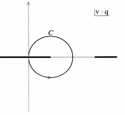
Figure 3.1: The integration contour C in the complex f. plane. The cuts extend to

Re E ---+

±CXJ

.

first cut arises from inserting the states between the two currents in the product Jt J,

and the second cut arises from inserting the states between the currents in the other

time ordering J Jt. So we arrive at

(3.9)

The sum over X includes the usual phase space factors, i.e., d3_p/(27r)3 _{for each particle}

in the state X.

Consider the integral of the product of a weight function w~(E) with

Tµv(E)

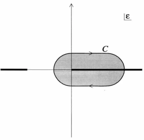
along

the contour C shown in Fig. 3.1. Assuming W is analytic in the shaded region

[image:35.539.161.395.60.287.2]

The maximum X mass on the right-hand side of Eq. (3.10) is determined by where

the contour C pinches the real axis. For convenience this mass is chosen to be less

than 2mb

+

me to prevent the occurrence of states X with b,

b,

and c quarks. We

take the maximum X mass to be 2mB and then Eq. (3.10) relies on local duality [21]

at this scale. Hereafter it is understood that sums over X only go over states up to

mass 2mB.

We require that: ( i) the weight function W ~ be positive semidefinite along the

cut so that every term in the sum over X on the right-hand side of Eq. (3.10) is

non-negative;

(ii)

W~(O)

= 1;

(iii)

w~

be flat near t: = 0, i.e.,

dW~(t:)/dt:J,=o

= O;

(iv)

and that it falls off rapidly to zero for t:

>

D.. We want to take D. ~

m

c

,b

·

Then

states X other than the D* give a contribution to the right-hand side of Eq. (3.10)

that is suppressed by (1/mc,b) 2. However, in our numerical results we consider D.

as large as 2 GeV. Although our analysis holds for any weight function that satisfies

these four properties, for explicit calculations we use

w(n)(t:) - _D._2n_

~ - E2n

+

,6. 2n ' (3.11)

with n = 2, 3, ... (for n = 1 the integral over t: is dominated by contributions from

states with mass of order m_{8 ).} These weight functions have poles at t: = 2

V"=T

D..,

therefore, as long as n is not too large and D. is much larger than the QCD scale,

AQco, the contour in Fig. 3.1 is far from the cut until t: is near 2mB. Then we should be able to calculate the integral in Eq. (3.10) using the operator product expansion

to evaluate the time ordered product.

The choice of the set of weight functions in Eq. (3.11) is motivated by the fact

that for values of n of order unity all poles of wln) lie at a distance of order D.

away from the physical cut. In this case the integral along the contour C can be

computed assuming local duality at the scale 2mB. The dependence of our results

on this assumption is extremely weak, because for D. ~ mB the weight function

is very small where the contour C touches the cut. As n --+ oo, wln) approaches

up to excitation energy .6.. with equal weight. Then the poles of

win)

approach the

cut, and the contour C is forced to lie within a distance of order b../n from the cut

at E

=

.6... In this case the evaluation of the integral along the contour C relies also

on local duality at the scale .6... 3

Neglecting perturbative QCD corrections and nonperturbative effects

correspond-ing to operators of dimension greater than five, the operator product expansion gives

[31)

~

T:4A

= -~ + (.\1 + 3.\2)(mb - 3me) _ 4.\2mb - (.\1 + 3.\2)(mb - me - t:) ( 3.12)

3 t i E 6m~t:(2me+t:) mbt:2 (2me+t:) '

when Jµ

=

Aµ

=

C/µ/5 b, and

~ T-VV = _ 1 + (.\1 + 3.\2)(mb + 3me) _ 4.\2mb - (.\1 + 3.\2)(mb - me - t:)

3 t i 2me+E 6m~t:(2me +t:) mbt:(2me+t:) 2 '

(3.13)

when Jµ = Vµ = C/µ b. Performing the contour integration yields

~

L

w~[(mx

- me) - (mB - mb)] (27r)3 83(px)

l(XIA;IB)l

2 x

=

1 __

.\2 +

(.\1

+ 3.\2)

(-1

+ _1 + _ 2 _)

m~ 4 m~ m~ 3memb ' (3.14)

~

L

w~[(mx

- me) - (mB - mb)] (27r)3 83(px) l(XIVilB)!2

x

(3.15)

These equations hold for any W ~ that satisfies the four properties mentioned above.

Higher order terms in the operator product expansion for T;; give contributions with

more factors of 1/t: on the right-hand sides of Eqs. (3.12) and (3.13). Therefore, if

the weight function has nonvanishing m'th derivative at E

=

0, there are corrections

to the right-hand side of Eq. (3.14) of order

(3.16)

We require that ~ be large enough compared with Aqco so that such terms are smaller than those we kept in Eq. (3.14). For m

>

1, ~ can still be smaller than

rnc,b· Higher order terms in the operator product expansion of T:fV give corrections

to the right-hand side of Eq. (3.15) of order (Aqco/mc,b)2 _{(Aqco/ ~r-}1_.

This is why

we imposed condition

(iii).

For the weight function

wl_n)(c)

in Eq. (3.11) the first

nonvanishing derivative is at m

=

2n.

We have considered the nonperturbative contributions to the sum rules

charac-terized by

>.

1 and

>.

2 . There are also perturbative corrections suppressed by powers

of the strong coupling. These are most easily calculated not in the operator product

expansion, but by directly considering the sum over states in Eqs. (3.14, 3.15) and

replacing the hadronic states by quark and gluon states. The perturbative corrections

are of two types. There are corrections of order as( mc,b) not suppressed by powers of

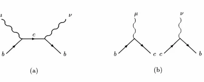
~/mc,b· These arise, at the parton level, from the final state X = c and change the term 1 on the right-hand side of Eq. ( 3 .14) to

rd.

There is another class of perturbative QCD corrections coming from final states

X that contain a charm quark plus additional partons, e.g., cg, cqq, etc. They

give a contribution to the right-hand side of Eqs. (3.14, 3.15) which is of order

[as(~)+

... ]

F(~), where the ellipses denote terms of higher order in the strong

cou-pling constant as, and for small~' F(~),...., ~2_{/m~,b· We have evaluated the strong}

coupling constant at the scale~' because this scale characterizes the typical hadronic mass in the sum over X. Note that, although these corrections are suppressed by

powers of ~/mc,b, they can be as important as the other perturbative corrections we considered since the strong coupling constant is evaluated at a lower scale ~- The

value for these corrections depends on the precise form of the weight function. We

use the ones given in Eq. (3.11). Such perturbative corrections were calculated in

[image:39.541.80.492.394.628.2]

b

b

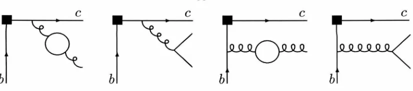
Figure 3.2: Feynman diagrams that contribute to the order a3(6.) corrections to the sum rules. The black square indicates insertion of the b ~ c axial or vector current.

the step-function 0(6. -

E)

(corresponding to

wl

00

l). As already pointed out, the use

of such a weight function relies on local duality at the scale

D.,

so the corrections

are expected to be less than those stemming from win) with small n relying on local

duality only at the scale 2mB. For n

2:

2 the order a8(6.) terms coming from the

Feynman diagrams in Fig. 3.2, and the order a;(D-) (30 terms arising from the

dia-grams in Fig. 3.3 were computed in Ref. [26]. The rationale for computing only the

part of the

a;

contribution proportional to (30 is that in most known examples it is

the dominant part of the full

a;

contribution. Taking into account these perturbative

corrections, Eqs. (3.14, 3.15) become

~

2:

Win)[(mx -

me) -

(mB -

mb)] (27r)3

83(px)

l(XIAilB)l

2

x

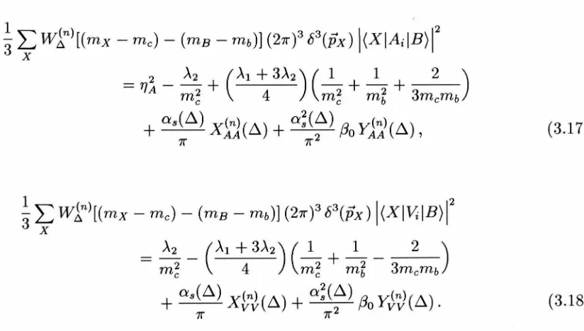
(3.17)

(3.18)

[image:40.539.78.491.43.134.2]

b

b

b

b

Figure 3.3: Feynman diagrams that de