Cavitation Inception In Separated Flows
Thesis by Joseph Katz
In Partial Fulfillment of the Requirements for the Degree of
Doctor of Philosophy
California Institute of Technology Pasadena, California
1982
-ii-Acknowledgment
I would like to express my deepest gratitude and appreciation to my advisor Dr.A.J.Acosta for his guidance and support during the course of the present research, and for his friendship, encouragement and assis-tance in the times that they were extremely needed.
Special thanks go also to Elton Daly and Joe Fontana for their help in the design and the machining of the present experimental equip-ment, and for their tireless efforts to make the life in the laboratory as easy as possible. I would also like to thank Dr.H.Shapiro for the design of the electronic equipment; G.Lundgren for the machinin9 of some of the test bodies; and R.Eastvedt, L.Montenegro and R.Relles for their help with the experiments. My thanks go also to B.Hawk, S.Berkley and R.Dudek for their help with the administrative details and for the prep-aration of the thesis manuscript.
I would like to acknowledge the financial support of the Naval Sea System Command General Hydrodynamic Research Program administered by David W.Taylor Naval Ship Research and Development Center.
-iii-ABSTRACT
The phenomenon of cavitation was studied on four axisymmetric bodies whose boundary layers underwent a laminar separation and sub-sequent turbulent reattachment. The non-cavitating flow was studied by holography and the Schlieren flow visualization technique. Surface distributions of the mean and the fluctuating pressures were also measured. The conditions for cavitation inception and desinence were determined and several holograms were recorded just prior to and at the onset of cavitation. The population of microbubbles and the nature of the subsequent development of visible cavitation was deter-mined from the reconstructed image.
High rms and peak values of the fluctuating pressure were measured (up to 90 percent of the dynamic head), the negative peaks being larger than the positive ones except for the reattachment zone where large positive peaks existed. The power spectra contained peaks thought to originate within the large eddies of the mixing layer and in one case there were also peaks due to the laminar boundary layer instability waves.
-iv-between the surface minimum pressure and the cavitation inception indices also indicated that inception could not occur near the surface of the bodies having a large separation region.
The appearance of visible cavities was preceded by the appearance of a cluster of microbubbles only in the cavitation inception region. The nuclei population in the other sections of the flow field remained fairly uniform. This observation supports the assumption that cavita-tion is initiated from microscopic free stream nuclei. The rate of cavitation events was estimated from the nuclei population and from the dimensions of the separation region. It was shown for one of the bodies that at least one bubble larger than 10 micrometers radius was exposed every second to a pressure peak which was sufficiently large
-v.;..
Chapter I - Figure Captions
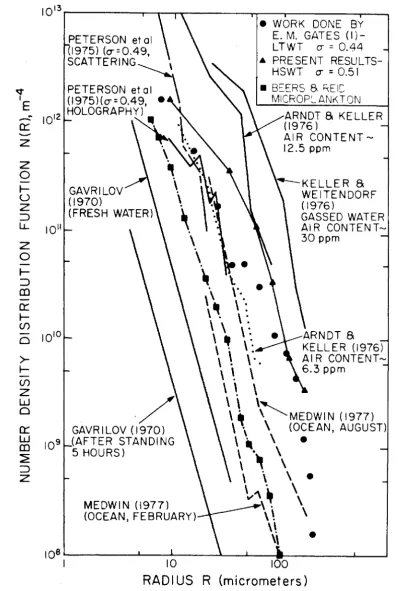
1.1 Nuclei distribution from various sources, The data of the HSWT and Beers et~ \1973) are superimposed on a graph presented by Gates and Acosta (1978).
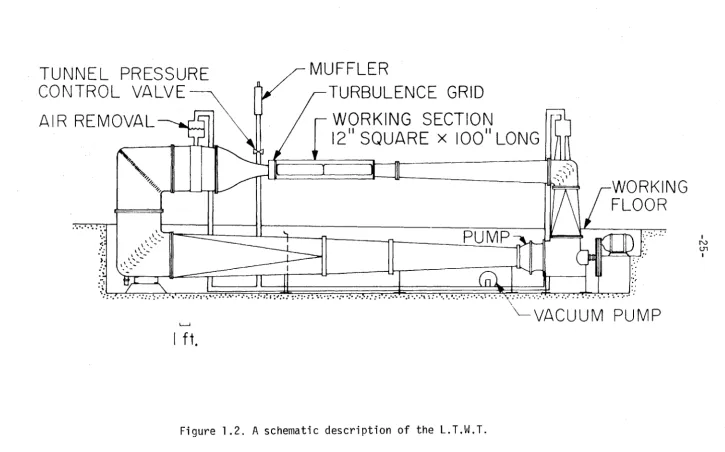
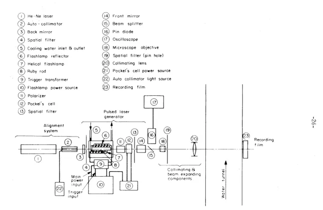
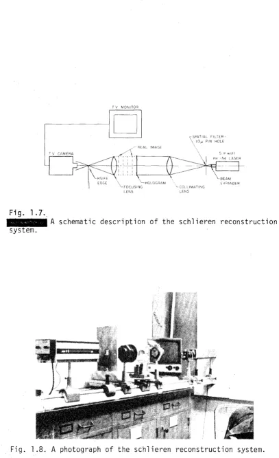
1.2 A schematic description of the L.T.W.T. 1.3 A schematic description of the holocamera. 1.4 A photograph of the holocamera.
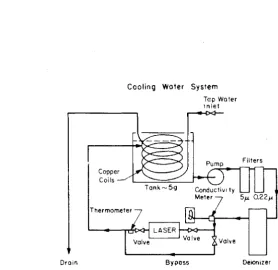
1.5 A schematic description of the laser cooling system.
-vi-Chapter II - Figure Captions
2.1 A schematic description of the blunt body with the pressure taps on its surface.
2.2 A schematic description of the different headforms with the pres-sure taps on their surface.
2.3 The pressure coefficient distribution on the surface of the two inch blunt body.
2.4 The separation zone minimum pres-sure coefficient on the two inc~
blunt body.
2.5 The pressure distribution on the surface of the blunt body in various cavitation indices and in the same velocity,
2.6 The pressure coefficient distribution on the surface of the hemis-pherical body.
2.7 The pressure coefficient distribution on the surface of the step body.
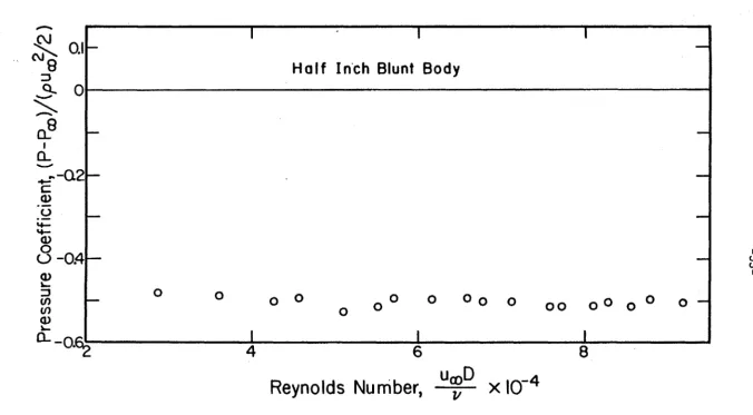
2.8 The pressure coefficient at
x/D
~ 0,5 on the one-half inch blunt body plotted against the Reynolds number.2.9 A combined series of schlieren photographs displaying the entire separation and reattachment zones on the surface of the two inches blunt body.
2.10 A schematic illustration of the injection points, the jets and the separation zone on the two inch blunt body that is shown in Figure
2.9~
-vii-the.blunt body showin~ the injection points at: a) x/D = 0.1, 0.25 and 0.45; b) x/D = 0.45, 0.75 and 1.0; c) x/D
=
1.0, 1.25 and 1.5; d) x/D=
1 .5, 1.75 and 2.0; e) x/D=
2.0, 2.25 and 2.5. 2.12 A schlieren photograph of the injection points at x/D=
1 .5,1.75 and 2.0 when the upstream jets are clo~ed.
2.13
A
laser shadowgraph of the flow around the two inch blunt body,5
Re D
=
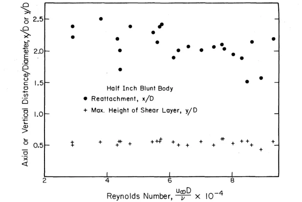
1 . 1 x 1 0 .2.14 The height of the mixing layer boundary and the reattachment length on the two inch blunt body.
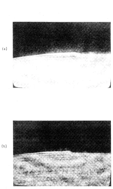
2.15 Laser shadowgraphs of the flow around the blunt body in a very low velocity; a) u = 0.5 ft/sec; b) u = 1 .5 ft/sec. co co
2.16 A reconstructed hologram of the separation and transition regions on a heated two inch blunt body; uco = 4.7 ft/sec.
2.17 Laser shadowgraphs of the flow around the one-half inch blunt body. a) u = 18.5 ft/sec; b) u = 14.3 ft/sec. co co
2.18 A sketch of the sbadowgraph that is displayed in Figure 2.17a. 2.19 The height of the mixing layer boundary and the reattachment
length on the one-half inch blunt body.
2.20 Two images of the same hologram displaying the separation zone
5
on the hemispherical body (uco = 11 .2 ft/sec, Re0 = l.8xl0 ); a) schlieren reconstruction; b) non-filtered image.
2.21 Two images of the same hologram displaying the separqtion zone
5
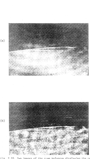
-viii-2.22 Two images of the same hologram displaying the separation zone on the hemi spheri ca 1 body ( uCXl = 2 3. 1 ft/sec, Re0 = 3. 7 x 10⁵ ) ; a) schlieren reconstruction; b) non-filtered image.
2.23 The location of separation and transition on the hemispherical body.
2.24 The height of the separation bubble on the surface of the hemispherical body,
2.25 Schlieren reconstructed holograms of the separation zone on the surface of the step body in various velocities: al um= 8,6
5 5
ft/sec, Re ~ l.4xl0 ; b} um= 10.9 ft/sec, Re0 = l,7xl0 ; c) u00
=
13~8
ft/sec, Re0=
2.2x1D5
; d) u00
=
16.1 ft/sec,5 Re0
=
2.6xlo •2.26 The location of separation and transition on the surface of the step body.
-ix-Chapter III - Figure Captions
3.1 A schematic description of the system for pressure fluctuation measurements.
3.2 Rrns values of the fluctuating pressure on the surface of the blunt body plotted against the Reynolds number.
3.3 Rms values of the fluctuating pressure on the surface of the blunt body
3.4 Probability density and distribution histograms of pressure fluctuations at x/D
=
0.328, u00=
18 ft/sec, Re0
=
3.0x10 5.
3.5 Probability density and distribution histograms of pressure fluctuations at x/D
=
0,578 and Re0=
3.0xl05 displaying the effects of signal filtering. Sampling time is 12 seconds. 3.6 Probability density and distribution histograms of pressurefluctuations at x/D
=
l.078 and Re0=
2.85xlo5 displaying the effects of filtering when the sampling time is 102 seconds. 3.7 Peak values of pressure fluctuations on the surface of the bluntbody at x/D
=
0.328.3.8 Peak values of pressure fluctuations on the surface of the blunt body at x/D
=
0,578.3.9 Peak values of pressure fluctuations on the surface of the blunt body at x/D
=
0.828,3.10 Peak values of pressure fluctuations on the surface of the blunt body at x/D
=
1.08.
-x-3.12 Peak values of pressure fluctuations on the surface of the blunt body at x/D
=
1 .578.3.13 Peak values of pressure fluctuations on the surface of the blunt body at x/D
=
l.828.3.14 Peak values of pressure fluctuations on the.surface of the blunt body at x/D = 2.078.
3.15 Axial distribution of the pressure fluctuation peaks on the surface of the blunt body. u00
=
8.8 ft/sec, Re0
=
l .4xl05. 3.16 Axial distribution of the pressure fluctuation peaks on thesurface of the blunt body. u00
=
14 ft/sec, Re0=
2.3xlo 5. 3.17 Axial distribution of the pressure fluctuation peaks on thesurface of the blunt body. u00 = 18 ft/sec, Re0
=
2.9xlo 5. 3.18 Axial distribution of the pressure fluctuation peaks on the5 surface of the blunt body. u00
=
21 ft/sec, Re0=
3.4xl0 . 3.19 Rms values of the fluctuating pressure on the surface of thestep body plotted ag~inst the axial location.
3.20 Rms values of the fluctuating pressure on the surface of the step body plotted against the axial location.
3.21 Axial distribution of pressure fluctuation peaks on the surface of the step body. u00
=
8.6 ft/sec, Re0=
1 .4xlo5•3.22 Axial distribution of pressure fluctuation peaks on the surface of the step body, u00
=
11.4 ft/sec, Re 0=
1.84xl05.3.23 Axial distribution of pressure fluctuation peaks on the surface
5
-xi-3.24 Axial distribution of pressure fluctuation peaks on the surface of the step body. u00
=
16.3 ft/sec, Re0
=
2.63x105.3.25 Axial distribution of pressure fluctuation peaks on the surface
5
of the step body. u00
=
17.9 ft/sec, Re0=
2.89xl0 .3.26 Axial distribution of pressure fluctuation p·eaks on the surface of the step body. u00
=
19.6 ft/sec, Re0
=
5 3.17xl0 .
3.27 Axial distribution of pressure fluctuation peaks on the surface of the step body. u 00 = 21.2 ft/sec, Re0 = 3.42xlo 5.
3.28 Axial distribution of pressure fluctuation peaks on the surface of the step body. u00
=
22.5 ft/sec, Re0
=
3.63xl0 . 53.29 Axial distribution of pressure fluctuation peaks on the surface of the step body. The signal is filtered with a high pass filter at 90 hz. u00
=
17.9 ft/sec, Re 0=
2.89xl0 . 53.30 Rms values of the fluctuating pressure on the surface of the hemispherical body plotted against the Reynolds number. 3.31 Rms values of the fluctuating pressure on the surface of the
hemispherical body plotted against the axial location.
3.32 Rms values of the fluctuating pressure on the surface of the hemispherical body plotted against the axial location.
3.33 Peak values of pressure fluctuations on the surface of the hemispherical body at x/D
=
0.519.3.34 Peak values of pressure fluctuations on the surface of the hemis-pherical body at x/D
=
0.556.
-xii-3.36 Peak va1ues of pressure fluctuations on the s·urface of the hemis ... pherical body at x/D = 0.659,
3.37 Peak values of pressure fluctuations on the surface of the hemis"" pherical body at x/D = 0.681.
3.38 Peak values of pressure fluctuations on the ·surface of the hemis-pherical body at x/D = 0.744,
3.39 Probability dens·ity and distribution hi·stograms of pressure fluctuations on the surface of the hemispherica 1 body.
5
x/D
=
0.609, Re0
=
3,75xl0 •3. 40 Probability dens Hy and distribution histograms of pressure fluctuations on the surface of the hemispherical body.
5
x/D = 0.609, Re0
=
3,13xl0 ,3.41 Spectrum of pressure fluctuations on the surface of the blunt body. x/D = 0.453 u00 = 21.2 ft/sec, a) 0-500 Hz, b} 0-100 Hz.
3.42 Spectrum of pressure fluctuations on the surface of the blunt body. x_/D = 1,203, u00 = 21 ,3 ft/sec. a} 0-500 Hz, b) 0 ... 100 Hz,
3.43 Spectrum of pressure fluctuations on the surface of the blunt body. x/D
=
1.953, u00 = 21 .2 ft/sec. a) 0~500Hz,
bl
0-100Hz,
3.44 Spectrum of pressure fluctuations on the surface of the blunt 5
body. x/D
=
0,453, u00 = 14.1 ft/sec, Re0=
2,3xl0 ,3.45 Spectrum of pressure fluctuations on the surface of the blunt body. x/D
=
1.203, u00=14.l ft/sec.3.46 Spectrum of pressure fluctuations on the surface of the blunt body. x/D
=
1.953, u =14.1 ft/sec. 00 •-xiii~
3.48 Frequency of the peaks in the spectra of pressure fluctuations at x/D
=
1.078 on the blunt body surface.3.49 Frequency of the peaks in the spectra of pressure fluctuations at x/D = 1.328 on the blunt body surface.
3.50 Spectrum of pressure fluctuations on the surface of the step
5
body. x1
/H
=
1.25, Re0=
2.63xlO .3.51 Spectrum of pressure fluctuations on the surface of the step
5
body. x'/H
=
9.8, Re0=
3.54xl0 .3.52 Spectrum of pressure fluctuations on the surface of the step
5
body. x'/H
=
14.53, Re 0=
3.63xl0 .3.53 A comparison between the step body spectral peaks and the estimated peak frequencies of turbulent fluctuations.
3.54 Spectrum of pressure fluctuations on the surface of the hemis-5 pherical body. x/D
=
0.556, u00=
12.6 ft/sec, Re0=
2.0xlO . 3.55 Spectrum of pressure fluctuations on the surface of thehemis-pherical_ body. x/D = 0,556, u00 = 17.4 ft/sec, Re0
=
2.8xl05. 3.56 Spectrum of pressure fluctuations on the surface of thehemis-- 5
pherical body. x/D
=
0.609, u00=
12.0 ft/sec, Re0 - 1.9x10. 3.57 Spectrum of pressure fluctuations on the surface of the
hemis-4 pherical body. x/D = 0,681, u00
=
6 ft/sec, Re0=
9.6xl0 . 3.58 Spectrum of pressure fluctuations on the surface of thehemis-5
pherical body. x/D
=
0.681, u00=
12.7 ft/sec, Re0=
2.lxlO . 3.59 Spectrum of pressure fluctuations on the surface of thehemis-5
pherical body. x/D
=
0.681, u00=
21.3 ft/sec, Re0=
3.4x10. 3.60 Calculated values of the hemispherical body boundary layer
-xiv-3.61 Calculated amplification of the laminar boundary layer waves in the separation point of the hemispherical body.
3.62 Frequency of the peaks in the spectra of pressure fluctuations at
x/D
=
0.609 on the hemispherical body surface~ Alsoincluded are the calculated peaks of the boundary layer waves. 3.63 A comparison between the hemispherical body low frequency peaks
-xv-Chapter IV - Figure Captions
4.1 A photograph of an early stage of cavitation on the two inch
. 5
blunt body Re
0
=
3.6xl0 , cr=
1.70.4.2
A
photograph of cavitation on the two inch blunt body.5
Re0
=
3.6xl0 , cr=
1.60.4.3 Holograms of the first microscopic signs of cavitation near the surface of the two inch blunt body. Re
0
=
2.3xlo5, a= 1.21. The 11large11 sheared bubbles are located at a) x/D= 0.89,
y/D
=
0.13; b) x/D=
0.96, y/D=
0.22.4.4 A hologram that displays the population of bubbles below and above the shear layer of the blunt body during cavitation in-ception. Re 0
=
2.3xl05, a= 1.15. The hologram covers theregion between x/D
=
0.23 and 0.45 and y/D = 0.11 and 0.27. 4.5 Maps of bubble population near the surface of the two inch bluntbody. a) Re0
=
2.83xlo5, a= 3.55; b) Re0=
2.94xl05, a= 3.00;. 5·
c} Re0
=
3.06xl0 , a=
2.56.4.6 The number density distribution function of bubbles that were counted near the surface of the two inch blunt body. The counted sections are defined by the dashed lines in Figure 4.5.
a) Re0 -- 2.85xl0 , 5 a= 4.74; b) Re
=
5D 2.83xl0 , a
=
3,55;c) Re 5 cr
=
2.99; d) Re=
5 a=
2,67; 0=
2.83xl0 , D 2.84xl0 ,e) Re0
=
2.99x10⁵, 0=
3.05; f) Re=
D
5
3.00xlO , a
=
3,04; g) Re 0=
2.94xl05, a=
3.00; h) Re D=
3.02xl05, a=
2.86;i ) Re0
=
2. 99xl05, a=
2.76;j)
Re=
5
-xvi-· 4.7 Cavitation inception indices on the two inch blunt body. 4.8 Cavitation desinence indices on the two inch blunt body. 4.9 A hologram of cavitation inception on the one-half inch blunt
4 body. u
=
21 .1 ft/sec, Re0
=
8.42xl0 , a= 1.41.4.10 A hologram of cavitation inception on the one-half inch blunt
4
body. u
=
21.1 ft/sec, Re0=
8.42xl0 , a= 1.41.4.11 Probability density histograms of the location of cavitation inception on the one-half inch blunt body. a) axial location,
b) vertical location.
4.12
A
description of the counted sample volumes near the surface of the one-half inch blunt body.4 .13 The population of bubbles near the surface of the one-half inch blunt body. u
=
21 ft/sec, Re0=
8.4x10⁵; a) a= 1.69;b) cr
=
1 . 59; c) a=
I, 58; dJ a=
1 • 52; e} cr=
1 . 51 , f) a=
I • 4b;g) a= 1.46; n) a= 1.78; i) cr
=
1.52.4.14 Cavitation inception indices on the one-half inch blunt body. 4.15 Cavitation desinence indices on the one-half inch blunt body. 4.16 Travel ling bubble cavitation on the hemispherical body.
5
Re
0
=
3.70xl0 , a= 0.73.4.17 Band type cavitation on the hemispherical body.
cr = 0.55.
5
= 3.70xl0 ,
4.18
A
mixture of band and travelling bubble cavitation in a tunnel5
-xvii-4.19 A hologram of cavitation inception on the hemispherical body. Re0
=
3xlo5, a= 0.607. The hologram covers the region between x/D = 0.53 and 0.67. (The flow is from left to right.)4.20
A
hologram of cavitation inception on the hemispherical body.5 .
Re0
=
3.77xl0 , a=
0,630. The hologram covers the region between x/D = 0.51 and 0.65.4.21
A
sheared free stream bubble above the separation zone of the hemispherical body. Re0
=
3,8xl0 5, a= 0.63. The width of the
screen is 6.9 mm and the bubble is located at x/D
=
0~55.4.22
A
hologram of band type cavitation on a heated hemispherical body. Re0=
3.3xlo5, a= 0.46. The width of the screen is 6.9 mm and cavitation separation is at x/D=
0.42.4.23 A hologram showing the laminar and cavitation separation points on the hemispherical body. Re0
=
3.54xl05, cr=
0.494. The width of the screen is 3.25 mm and cavitation separation is at x/D=
0.43.4.24 A hologram of travelling bubble cavitation on the he~ispherical body. Re0
=
3.8xl05, a= 0,63. the photograph covers the region between x/D = 0.32 and x/D = 0.46,4.25 A map of bubble population during cavitation inception on the hemispherical body. Re 0 = 3xl05, a= 0.607.
-xviii-4.27 A description of the counted sample volumes near the ~urface
of the hemispherical body.
4.28 The population of bubbles near the surface of the hemispherical
5 5
body. a) Re0
=
3.23xl0 , a=
0.550; b) Re0=
3,22xl0 ,a= 0.608; c} Re0
=
3.23xlo5, a= 0.611; d}~e
0
=
3~50x10
5,
a= 0.643; e} Re0
=
3,19xl05, a= 0.649; f) Re0
=
3.19xlo5 ,a= o.669; g) Re
0
=
3.3lxlo 5, a= 0.683; h} Re
0
=
3.76xlo 5,
a
=
0.586.4.29 Inception indices of travelling bubble cavitation on the hemis-pherical body.
4.30 Inception indices of band type cavitation on the hemispherical body.
4.31 Desinence indices of band type cavitation on the hemispherical body.
4.32 Bubble ring cavitation on the step body. Re - 5
0 - 3, 60xl
o ,
a= 1.10~4.33 Formation of band type cavitation on the step body( 5
Re 0
=
3. 60 x 10 , a=
0. 5 3.4.34 Inception of cavitation on a non-heated step body. 5
Re
0 = 2. 78 x 10 ,
o
=
1. 07. a) a tota 1 view of the cavitati ngzone; bJ a close-up view of part of the region extending from 3.5 to 10.5 mm behind the step.
4.35 Inception of cavitation on a heated step body.
a= 1.07.
5 Re
-xix-4.36 inception of cavitation on a heated step body. Re
0 =· 2.78x10⁵,
a= 1.11. a) a total view of the cavitating zone; b} a
close-up view of the region behind the step.
4.37 The region near the separation point of the hologram shown in Figure 4.36.
4.38 Inception of cavitation on a non-heated step body.
5
Re
0 = 3. 62 x 1 O , a= 1. 20.
4.39 Probability density histograms of the axial location of cavita-tion incepcavita-tion on the step body; a} Re
0
=
2.77xl05;5 · b) Re
0
=
3. 55 x 10 .4.40 A map of bubble population during cavitation inception on the
5
step body. Re0
=
2.78xl0 , a= 1.11.4.41 The population of bubbles near the surface of the step body during cavitation inception; a) Re0
=
2,8xl05, a= 1.11;5 5
b) Re0
=
2.78xl0 , o=l .11; c) Re0 = 2.78xl0 , a= 1.07 4.42 Cavitation inception indices on the step body,4.43 Cavitation desinence indices on the step body.
-xx-LIST OF SYMBOLS
a acceleration
the average pressure coefficient defined by (P-P )/(0.5 pu 2) 00 00 Cpsor CPB the average pressure coefficient inside the separation zore
I
cP
the rms pressure fluctuations coefficient defined by/;2;(o.5
pu:)
D body diameter
f frequency of fluctuations
maximum range of pressure fluctuations spectrum
. u . u
a calculated frequency defined by 0.56 Loo ; 0.56 Loo
1 2
the height of the separated bubble (separation stream line) h' the height of the separated bubble upstream of the step H the height of the step on the step body
L length of separation zone L
1 the distance between separation and reattachment defined
N(R)
n(R)
p
P'
p
by xr-xsep
the distance between transition and reattachment defined by xr-xtr
the distance between two neighboring vortices in a shear layer the length of the pressure transducer calibrating tank
the number of density distribution functions of nuclei the density of nuclei
static pressure fluctuating pressur~
-xxi-atmospheric pressure
the tunnel free stream static pressure vapor pressure in room temperature the pressure in the core of the vortex the flow rate of bubbles in the shear layer
the flow rate of bubbles that are exposed to pressure peaks bubble radius
dR/dt
r the radius of the pressure transducer the radius of a vortex core
u 00
D
body Reynolds number defined by
-V-u
e
momentum thickness Reynolds number defined by ~
*
u 0
00
displacement thickness Reynolds number defined by S distance along the surface of the body
St Strauhal number defined by fD/u00or
~=
T surface tensiont
8 characteristic response time of a bubble u local velocity
u 00 free stream velocity uAv average velocity
~u velocity difference across a shear layer uc convection velocity
x axial distance from the stagnation point x1
-xxii-xtr axial location of transition xr axial location of reattachment
xi axial location of cavitation inception
y a dimension normal to the body surface
*
o
boundary layer displacement thicknessow
shear layer slope thickness defined by6u/(~~)max
e
momentum thicknesses momentum thickness at separation
p water density
w frequency in rad/sec
r
circulationwavelength of eddies in the
a cavitation index defined by
a.
1 cavi ta ti on cavitation
inception index desinence index
shear layer
(P00-PV)/(0.5 pu ) 2
I
-xxiii-TABLE OF CONTENTS
ACKNOWLEDGMENT ABSTRACT
LIST OF FIGURE CAPTIONS LIST OF SYMBOLS
I NTRODUCTI or~ I.l BACKGROUND
I.2
I.1.1
I.1.2
I.1.3
I.1.4
I. l. 5
I. l. 6
Scale Effects in Cavitation Cavitation Nuclei
Cavitation Inception-Physical Models Viscous Effects on Cavitation Inception Remarks
Scope of the Present Work EXPERIMENTAL EQUIPMENT
I. 2. 1
I. 2 .2
I.2. 3
I. 2.4
I. 2. 5
l~ater Tunnel Test bodies
The Nuclei Counter-The Holography System The Holocamera
Reconstruction System FIGURES - CHAPTER I
Page ii iii v xx l 4 7 9 12 13 14 14 15 16 17 21 24
II A STUDY OF THE NON~ CAVITATING FLOW AROUND THE TEST BODIES 30 II.l AVERAGE PRESSURE MEASUREMENTS
II.1.1 Apparatus and Procedure II.1.2 Results
II.2 FLml VISUALIZATION
II.2.1 Apparatus and Procedure
30 30
32
34
-xxiv-TABLE OF CONTENTS (continued) II.2.2 Results - Blunt Noses
I I. 2. 3 Results - Hemi spheri ca 1 Nose I I. 2. 4 Results - Step Nose
II.3 DISCUSSION
FIGURES - CHAPTER I I
III PRESSURE FLUCTUATION MEASUREMENTS III.l APPARATUS
II I. 2 RESULTS
III.2.1 Blunt Nose
Page 36 40 41 46 75 75 78 78
II I. 2. 2 Step Nose 83
III.2.3 Hemispherical Nose 86
III.3 SPECTRAL MEASUREMENTS OF THE FLUCTUATING PRESSURE 91
III.4
III.3.1 Introduction
III.3.2 Apparatus and Procedure III.3.3 Blunt Nose
III.3.4 Step Nose
III.3.5 Hemispherical Nose DISCUSSION
III.4. 1 Comparison to other sources III.4.2 The Turbulent Spectral Peaks III.4.3 Low Frequency Fluctuations
III.4.4 Effect of Transducer Size on the Measurements
II I. 4 . 5 Summary FIGURES - CHAPTER I I I
-xxv-TABLE OF CONTENTS (continued) Page
IV CAVITATION PHENOMENA ·153
IV. 1 EXPERIMENTAL PROCEDURES 153
IV.1.1 Cavitation Inception and Desinence
Measurements 153
IV. 1. 2 Holographic and Photographic Methods 154 IV.2 OBSERVATIONS AND MEASUREMENTS OF CAVITATION
PHENOMHJA 155
IV.2.1 Two Inch Blunt Body 155
IV.2.2 Half Inch Blunt Body 158
IV.2.3 Hemispherical Body 161
IV.2.4 Step Body 167
IV.3 DISCUSSION: THE EFFECT OF BUBBLE POPULATION ON
CAVITATION INCEPTION 173
IV.3.1 Free Stream Bubble Population 173
IV.3.2 Conditions for Instability 177
IV.3.3 Response Time of Bubbles vs Spectra of
Fluctuations 178
IV.3.4 Rate of Cavitation Events 182
IV.3.5 Sumnary and Corrments 130
IV.4 DISCUSSION: THE EFFECT OF THE FLOW FIELD ON
CAVITATION INCEPTION 193
IV.4.1 Summary 193
IV.4.2 Cavitation and the Shear Layer Eddies FIGURES - CHAPTER IV
v
SUMMARY AND CONCLUSIONS 237REFERENCES 242
-1-I. INTRODUCTION I.l Background I.1.1 Scale Effects in Cavitation
Vapor and gas cavities are formed in a liquid either when there is sufficiently high temperature or when the pressure is reduced below a critical value. The former process is usually described as boiling, thermal effects being the main contributor, and the latter is defined as cavitation and is controlled by inertial or dynamic phenomena. A com-parison between these processes is made by Plesset (1949, 1956) and is reviewed also by Knapp et al. (1970).
The present work focuses on cavitation whose physical appearance can be either in the form of bubbles of various sizes and shapes, or in the form of large vapor (and gas) cavities that are attached to the sur-face of a body. Cavitation appears on ship propellers and on the
components of pumps, turbines, valves, and hydrofoils. It may become a major design problem due to its effect on the performance of hydraulic machinery and to its contribution to erosion and noise.
-2-cavitation research and part of the existing literature enclosed with this topic will be discussed in the following sections.
One of the major problems in fluid mechanics is to predict the characteristics of a prototype from the results of tests on a model. The common technique is to use similarity parameters thought to be appropriate which, together with known scaling laws, assist in extrapo-lating the model results to the full scale design. Insofar as cavita-tion is concerned, the scaling laws are not fully understood, as has been recently discussed by Acosta and Parkin (1975).
The basic parameter for cavitation experimentation is the cavita-tion index (or number),cr, defined as
p - p
00 v
a
=
1 2-2 p u
00
P and u being the characteristic pressure and velocity, respectively, 00 00
P the density, and Pv the vapor pressure of the bulk liquid. In the present experiments P00 aAd u00 are the conditions in the tunnel test sec-tion measured far from the body. There are two critical values of a;
the first one, a;, is the cavitation inception index determined by
reducing the tunnel pressure keeping the velocity constant until the first signs of cavitation appear. The second critical value is the
-4-I.1.2 Cavitation Nuclei
The weak spots or the cavitation nuclei that are essential to the onset of cavitation can originate either from the free stream or the surface of a body. The presence of the surface nuclei may be due to the material itself and the finish of the body surface .. Holl and Treaster
(1966), Holl (1968), Reed (1969), Gupta (1969), and Van der Meulen (1972a,b) have all studied this aspect of nuclei. These investigators tested stainless steel bodies with different surface fitiishes, Teflon, nylon, and glass bodies, and found significant differences between their inception indices and the appearance of cavitation. Acosta and
Hamaguchi (1967) found that a thin silicon oil coating (this oil dis-solves a large amount of air) on a body surface altered the inception indices first by increasing them when the layer was fresh and then by decreasing them (beyond the pure water results) after the coated body was submerged for a long time. Peterson (1968) measured the cavitation
inception indices for the very same body, first after exposing it to air and then by taking measures to remove the gas pockets from the sur-face. He found significant differences between the results, 0.78 for the former and 0.63 for the latter.
The effects of the surface quality and material and the signifi-cance of the pressure time history experienced by the body led some investigators (see Holl (1969))to suggest that cavitation is initiated from air pockets that were trapped in microscopic cracks and crevices that exist on the surface.
-5-gas bubbles, or solid particles that contain -5-gas pockets. The mathe-matical behavior of a spherical bubble that contains vapor and a noncon-densable gas is described by the Rayleigh-Plesset equation (see Plesset and Prosperetti (1977)) from which the conditions for equilibrium and instability can be developed (the latter will be discussed in Chapter 4). Epstein and Plesset (1950) showed that gas bubbles will disappear
by mass diffusion in an undersaturated liquid, and this conclusion led
several investigators to propose various explanations for the presumed existence of gas bubbles or nuclei in liquids. Some of these are dis-cussed by Plesset (1969), but Harvey et al. (1944, 1947) appear to pro-vide the most tenable suggestion, namely, that gas is contained within cracks on the surface of microscopic solid particles. This physical mechanism has attracted much attention (see, for example, Keller (1972, 1973)) but a direct observation has not yet been possible.
The importance of these nuclei as a source of nucleation has led to the development of several detection or observation techniques. These include the microscopic observations of water samples, the 11
Coul-ter counCoul-ter,11
"single particle light scattering," the "acoustic" tech-niques for detection of gas bubbles, holography with microscopic obser-vation of the reconstructed image, and finally, the liquid quality meter (Oldenziel (1979)). These different detection techniques are discussed by Godefroy et al. (1981), Gates (1977), and Morgan (1972).
-6-(1962, 1964) and Schiebe (1969) applied an acoustic method to measure the undissolved gas content in test water and thereby obtained an esti-mate of the concentration of microbubbles. For other reasons the pre-dicted rate of cavitation events compared poorly with measured data. Keller (1972, 1973) determined the nuclei population by using a single particle light scattering device (the sample volume was illuminated by a He-Ne laser). This technique could not distinguish between solid par-ticles and bubbles, but Keller came to the conclusion that most of the detected nuclei were solid by comparing his results for various types of prepared test water (filtering and degassinq). He then pursued the Harvey nucleus model to show that this concept would explain a part of his experimental findings.
Only a few investigators have applied holography to cavitation nuclei detection, namely, Peterson et al. (1975), Feldberg and Shlemen-son (1973), Gates and Acosta (1978), and Billet and Gates (1979). This method, however, has been extensively used in aerosol measurements
(Thompson et a 1 ~ ( 1967)) ·and even for i dent i fi cat ion of p 1 an kt on (Beers et a 1.
(1973)). The holographic technique is widely used in the present study and the system used for this purpose will be described later.
-7-would seem plain that this difference could create significant "scal-ing" errors while applying laboratory results to field cavitation phenomena. Also note that the nuclei in the Caltech HSWT are found to be mostly solid particles, while the Caltech LnJT contains mainly free stream bubbles. This difference may explain why it is easier to cavi-tate the same body in the LTWT (provided that the flow is nonseparat-ing) while the liquid in the HSWT can support a certain tension (Gates and Acosta (1978)).
I.1.3 Cavitation Inceptio·n-Physical Models
There have been several attempts to develop a detailed theory that will explain the occurrence of cavitation near the surface of a streamlined body. One of the earliest models was that of Parkin (1952) who used the Rayleigh-Plesset equation and the known pressure field around a test body to determine the behavior of air and vapor nuclei that were stabilized on small solid particles in the liquid. Later Parkin and Kermeen (1953) carried out a series of experiments on a hemispherical headform body. They came to the conclusion that cavitation is sustained by small bubbles that grow at a fixed point in the body boundary layer until they are large enough to be entrained by the flow, travel downstream, and appear as macroscopic cavitation.
Parkin1
s theory was extended by Holl and Kornhauser (1969) to include the effects of initial conditions, stream and surface nuclei, thermodynamic effects of bubble growth, and the existence of a boundary layer. Van der Walle (1962) w,as motivated by Parkin and Kermeen 1
-8-in the boundary layer under the action of the body pressure gradient, adhesion forces to the surface, and viscous drag. Oshima {1961) made ari attempt to develop scaling laws with the help of assumed similarity laws and by claiming that cavitation inception took place when the bubble diameter grew to one-half the size of the boundary layer dis-placement thickness. These theories were based on Parkin and Kermeen's (1953) interpretation of their own experiments on the hemispherical body, and as will be discussed later, they ignored the most important phenomenon, namely, the existence of a laminar separation bubble on this body. A theory in which viscous effects were neglected was devel-oped by Johnson and Hsieh (1966). They calculated the trajectories and the stability of bubbles near the minimum pressure region on a body surface from which they developed the conditions for cavitation incep-tion. This theory was used by Schiebe (1969), whose work was mentioned earlier, while trying to estimate the rate of cavitation events with the acoustically-measured bubble population. Schiebe's results showed only qualitative agreement with experimentally measured values.
Keller's (1972, 1973) model that was also mentioned earlier is based or. the potential pressure field. He attributed the disagreement between his theory and the experimental results to viscous effects inside the pore of Harvey's solid nucleus.
The effect of diffusion of dissolved gas into a bubble during its motion in the supersaturated sections of the flow field (where the
-9-process defined as gaseous cavitation) but the rate of such bubble growth is on the order of seconds (see Epstein and Plesset (1950)) uhlike the dynamic bubble growth (vaporous cavitation) that occurs in milliseconds (see Knapp et al. (1970)). Oldenziel (1979) subsequently made additional calculations of gas diffusion during vaporous cavitation growth and
showed that a significant amount of gas is actually released into the bubble and thus his results suggest that these processes, that is, the gaseous and the vaporous cavitation, cannot be totally separated.
All the above theories deal with the behavior of a nucleus near the surface of a streamlined body exposed to the pressure field there. These models do not bring into full consideration several real-fluid flow phenomena such as the laminar boundary layer separation and the subsequent development of an unstable shear layer and turbulent reat-tachment. These phenomena are known to take place on many surfaces of interest.
I.1.4 Viscous Effects on Cavitation Inception
It was not until recently that the effect of viscous phenomena on cavitation was demonstrated by Arakeri and Acosta (1973, 1974, 1976) and Arakeri (1973) who applied the schlieren technique to observe the flow and the inception of cavitation on submerged axisymmetric bodies. They found that the laminar boundary layer on the surface of the
-10-away by the main external flow. Other bubbles were observed to grow at a fixed point inside the separation zone until they were large enough to be carried downstream. This form of cavitation disappeared when the pressure was lm~ered slightly to be replaced by a clear attached 11
band11
type cavity. This sequence of events is also demonstrated by Gates (1977) with a series of schlieren photographs and by Van der Meulen (1976) with a series of reconstructed holograms.
Arakeri and Acosta (1976) proceeded with their experiments and re-moved the separation bubble either by tripping the boundary layer in order to enforce early transition, or by increasing the free stream velocity. They found that as the laminar separated zone disappeared the clear band type cavity became unstable, patchy, and intermittent until no form of attached cavity could be maintained on several test bodies. These observations demonstrate clearly that for those bodies that possess a separated bubble, cavitation phenomena are closely related to the characteristics of this separation zone. Arakeri et al. (1978) demonstrated this relation also on a 1/8 caliber ogive body. They showed that a sudden change in the dimensions of the separation zone
(when the separated bubble bursts) causes also a large change in the cavitation inception index.
-11-group is the sharp edge disk tested by Kermeen and Parkin (1957). They observed that the first cavities appear within the shear layer, and further suggested that cavitation inception occurs in the core of the vortices in the mixing zone. This group is characterized by a strong dependence of the inception index on the Reynolds number.
The second group includes the bodies with a smaller separated zone where the neighboring surface affects the development of the mix-ing layer. Cavitation inception occurs near the reattachment zone due to the large pressure fluctuations there. This last statement is supported by Arakeri (1975a) and by Huang (1979) who measured the fluc-tuating pressure on the surface of the hemispherical nose body and found pressure peaks of 25 and 45 percent of the dynamic head, respec-tively. The cavitation inception index shows a weak dependence on the Reynolds number and its value is close to the absolute value of the pressure coefficient in the separated zone.
The third group includes the bodies with a very small separated bubble such as the ITTC headform (Arakeri {1973)) and is characterized by a cavitation index that is independent of the Reynolds number, and his upper bound is the absolute value of the pressure coefficient in the separation zone. The fourth group includes those cases where the laminar boundary layer undergoes natural transition to turbulence with-out separation. This group is characterized by a relatively low
-12-Meulen (1976)) and a series of headforms that were tested by Huang (1979).
Being motivated by his suspicion that the height of the separated zone plays a dominant role in cavitation phenomena, Arakeri (1979) proceeded by artificially changing this height by means of a small downstream-facing step at the tangency point of the hemispherical body. His results show that the dependence of the inception index on the step height (remarkably large changes in cr) is limited to small steps
(H/D ~ 0.01) beyond which the cavitation number reaches an asymptotic value that depends only on the Reynolds number. Another example of the effect of the dimensions of the separation zone is that of Van der Meulen (1980) on two hydrofoils at various angles of attack. His holo-graphic study of the flow displays the transition from a small separated zone at small angles of attack (similar to the second group in Arakeri and Acosta's (1979) classification) to the large scale eddies in the shear layer at large angles (similar to the first group). As a result, the cavitation inception 'indices display a growing dependence on the Reynolds number, and the physical appearance of the cavities changes from traveling bubbles to band type and then to the intermittent shear layer cavities as the dimensions of the separation zone are increased. I.1.5 Remarks
The preceding short introduction forms the background to the present work whose scope will be described in the following section. More extensive, older material can be found in the book by Knapp et al.
-13-a recent st-13-ate of the -13-art review on c-13-avit-13-ation is provided by Arndt ·(1981) and two earlier reviews by Acosta and Parkin (1975, 1980).
I.1.6 Scope of the Present Work
The present work focuses on cavitation in separated flows, that is, those cavitation phenomena that occur near the surface of a body whose boundary layer undergoes laminar separation followed by transi-tion in the shear layer and turbulent reattachment.
The first step will be to study the flow around the test bodies selected. This will be accomplished with holography and schlieren photography that will help in visualizing the flow patterns under fully wetted and cavitation inception conditions. Then the average pressure coefficients and the surface pressure fluctuations will be carefully measured (including the rms, peak values, and spectral distributions). The results will assist us in relating the location and the physical appearance of cavitation to flow phenomena such as the location and the dimensions of the separated bubble, the position of transition and reattachment, the eddy structure in the shear layer, and the location of high pressure fluctuations. The pressure field may also help ex-plain the relatively high cavitation inception indices that character-ize these separated flows.
-14-follow the development of cavitation from the micro to the macro (visi-ble) scale in order to provide direct evidence that the detected nuclei are the source of the large cavities. Some of the major parameters . that affect the nuclei population will also be studied, in particular the effect of the pressure-time history of the water in the test facility and various experimental procedures.
The discussion that follows the presentation of the results includes an attempt to estimate the rate of cavitation events around the present bodies by combining some of the major contributing factors. These factors include the nuclei population and size distribution, the negative pressure fluctuation peaks, their probability of occurrence, their frequency, and the location and dimensions of the observed cavi-tation inception region.
I.2 Experimental Equipment
The following section contains a description of the water tunnel, the test bodies, and the holographic system. The rest of the experi-mental equipment and test procedures that apply only to a certain experiment will be described in each chapter separately.
I.2.1 Water Tunnel
All the experiments were carried out in the Low Turbulence Water Tunnel (LTWT) whose schematic description is displayed in Figure 1.2. This facility is described in detail by Gates (1977) and only some of its main features are presented here.
-15-and 12 inches wide at the exit. The square settling (stagnation) chamber has a cross section of 48 by 48 inches, resulting in a contraction ratio . of 16:1. This chamber is equipped with two honeycombs and three damping screens that contribute in reducing the test section turbulence level to about 0.04 percent.
The water in the tunnel is pumped by a mixed-flow type pump that is driven by a 30 HP d.c. electric motor through a belt drive. The result-ing maximum velocity in the test section is fairly low ,about 24 ft/sec.
The pressure is controlled with a Nash 5 HP vacuum pump that is con-nected to a tank located above the settling chamber and a bypass valve to the atmosphere that is connected to the vacuum line.
I.2.2 Test Bodies
Four stainless steel axisymmetric bodies were tested in the present experiments. The first two bodies had a flat blunt nose but a different size. The first one was two inches in diameter and the second was one-half inch in diameter. The oth'er two bodies had a hemispherical headform, both two inches in diameter, the first with a smooth tangency, and the second with a one-millimeter downstream facing step at the tangency point. (This
last model will be referred to as the step body.) The bodies were mounted on a two-blade sting support and were 13 inches 1 ong and thus the nose was located 6.5 diameters upstream of the sting.
-16-fluctuation measurements (see Chapter 3) and the third one had a smooth, polished surface for the ca vi ta ti on tests. A detailed description of each of these headforms is provided in the following chapters.
I. 2. 3 The Nuc 1 ei Counter - The Ho 1 oqraphy Sys tern
Holography is the only existing technique that allows direct observa-tions of microparticles and bubbles in a moving liquid, and thus to know their exact shape and size. In this method, a three-dimensional image of a sample volume is reconstructed and all the observations are made in this image. The measurements can be made in any part of the sample volume and in almost any desired magnification.
A corrmon photographic record contains information about the intensity of the light scattered from a certain object. The hologram, however, con-tains also information about the phase dffference between the radiation from the object and a reference wave. This information is stored on a film in the form of an interference pattern, and a proper technique can be used to relocate any object to its original position in space.
Recording and Reconstruction. The hologram is recorded in the exper-imental facility. A desired sample volume is illuminated by a beam of collimated, coherent, and semimonochromatic light. The light diffracted from any object in this volume interferes with another coherent reference beam, and the resulting pattern is recorded on film. The technique used in the present study is the lensless Fraunhofer holography that is limited to holograms recorded in the "far field11
-17-becomes the reference wave that interferes with the light diffracted from the objects. The resulting pattern is recorded on a high resolution film that is located on the other side of the sample volume.
The developed holographic record is illuminated by another colli-mated coherent light source. While passing through the hologram whose transmittance is proportional to the recorded interference pattern, the reconstruction light is diffracted to create a three-dimensional image of the original volume. Actually, two images are created, a real and a virtual one. They are formed symmetrically on both sides of the hologram plane and have the same axis. The far field requirement in Fraunhofer holography insures that the virtual image will produce only a weak and almost uniform background illumination in the real image plane. A detailed analysis of this technique is described in chapters two and eight of
Co 11 i er et a 1 ( 1 9 71 ) .
The recording light source in the present system is a pulsed ruby laser. The use of such a laser is essential while recording a hologram of a moving object due to the high intensity required for a very short ex-posure time. The reconstruction light source is a five mw CW He-Ne laser. The difference between the wavelength of the lasers, 0.6943 µm of the ruby and 0.6328 µm of the He-Ne laser does not change the dimensions in the plane normal to the illumination axis but does affect the axial dimension. 1.2~4 The Holocamera
-18-recording film, and an alignment system.
Laser Cavity. A three-inch long, quarter-inch diameter cylindrical ruby rod is 11
excited11
by a helical xenon flashlamp. The ruby is located in a 22-inch long optical cavity created by two flat mirrors. The back mirror is a 100 percent reflecting dielectric surface, and the front one is a sapphire etalon ( z60 percent reflectivity). The front mirror also plays a role in longitudinal mode control of the laser. Two iris apertures located inside the cavity keep the light beam sufficiently narrow to avoid generation of multiple transverse modes.
The ruby rod and the flashlamp are located inside a sealed box whose interior is filled with filtered and deionized cooling water. The flash-lamp is covered with a highly reflecting cylindrical surface made of aluminum sheeting. This reflector insures that most of the flashlamp's light will be directed toward the center where the ruby is located.
When the laser is triggered, approximately 1000 joules that are stored in loaded capacitors discharge through the flashlamp. The flash is
initiated by a high voltage pulse generated from a different capacitor and magnified by a series injection trigger transformer. This high voltage, more than 20,000 volts, is needed for ionizing the xenon in the flashlamp, and thus activate the discharge of the main power whose voltage is only 3500 volts. The duration of the flash is more than one millisecond.
''Q Switching. 11
The amount of energy that is suppl i ed to the sys tern and the duration of the flash are sufficient for generating several laser pulses. In order to control the number of these pulses, the laser has to be 11Q switched 11
-19-calcite glan laser polarizer are used for this purpose. The switching system is located inside the cavity between the ruby and the front mirror.
The KD*P crystal introduces a retardation between the two mutually orthogonal components of the input field that is proportional to the voltage applied to it. I~ the present system the Pockels cell is loaded with 1.8 KV, a potential that is sufficient to cause a retardation of a quarter wave-length. After being emitted from the ruby the light is polarized by the glan polarizer and enters the crystal. While passing through the Pockels cell, ·a retardation of quarter wavelength is introduced and after reflection from the back mirror the light is retarded again by the same amount. As a result, the plane of polarization is rotated by 90°, and this light will be deflected by the glan polarizer. This Q switch prevents the oscil-lations of light in the cavity and the syste~ cannot lase.
In a prescribed time the voltage on the Pockel 1
s cell is dropped to zero for a very short duration. Since the crystal does not alter the polarization in this period, the light can oscillate in the cavity. This 1 i ght and the continuous lY. added energy from the fl ashl amp bring the ruby
to a critically excited state that results in the emission of a large laser pulse. The duration of this pulse is between 20 and 50 nanoseconds. If the cavity is switched more than once, two (or more) laser pulses will be emitted, thus the sytem can be applied for interferometry.
-20-Cooltng. Efficient cooling of the laser head is required due to the sensitivity of the ruby and the flashlarnp to small temperature changes. The cooling water is injected from six orifices that are located between the rod and the flashlamp at the rate of one gpm. As illustrated in Figure 1.5, the cooling system consists of a five-gallon storage tank, a pump, two filters (for 5.0 and 0.22 micron particles) and a deionizer. A conductivity meter located before the entrance to the laser head indi-cates the quality of the water before use. To prevent any scale deposit on the ruby rod and the flashlamp, the water is recirculated through the deionizer several times, bypassing the laser to provide a resistivity of at least 18 M cm (much less than 0.1 ppm of any contamination). The deionizer also cleans the water continuously during the operation.
Brass coils in which tap water flows are located inside the storage tank. This heat exchanger removes the heat from the cooling water.
The electronic power supply and control system were built by Shapiro Scientific Instruments. The mechanical components, the mounts, and the laser head assembly were designed and manufactured at Caltech.
-21-Since the intensity of the laser is much higher, the cavity output is at-tenuated by a neutral density filter.
Alignment. The alignment system consists of an autocollimator and a 0.5 milliwatt CW He-Ne laser. The autocollimator assists in aligning the laser cavity components which are mounted on carriers that can be carefully adjusted. The He-Ne laser helps in bringing all the components to a common axis and in positioning the pinhole in the focal plane of the objective.
I.2.5 Reconstruction System
After developing the film, the hologram is mounted on the reconstruc-tion system. The light source is a 5 milliwatt CW He-Ne laser whose output is expanded by an objective, spatially filtered by a pinhole, and
col-limated by a lens. The resulting beam illuminates the hologram, and the diffraction pattern caused by the film transmittance creates a
three-dirnensiona1 image of the original volume. A magnifying system, positioned inside the image field, focuses any desired cross section on a TV vidicon and the image can be seen on the screen of a monitor. The hologram is mounted on an x-y-z vernier carriage so that any point in the reconstruc-tion field can be focused on the vidicon.
-22-the principles of holography with -22-the schlieren effect. Instead of simply magnifying the image it is first focused to a point by the lens on the knife edge located in the focal plane. Most of the backward illuminating light source is thereby cut off and only the diffracted light can propagate downstream. The resulting schlieren effect is recorded by the vidicon and displayed on the TV screen. This modification in the reconstruction proce-dure eliminates most of the background noise and a major part of the laser speckle. A few examples of the difference between the "filtered11 and 11
non-filtered11 reconstructed image are displayed in Figures 2.20 to 2.22. The main advantage of this technique over the conventional
schlieren system comes from the coherent recording light source that makes the diffraction pattern a first-order phenomenon unlike the common schlieren photograph recorded with a white light source. This difference allows one to record a hologram in the usual manner and to adjust the position of the knife edge only while reconstructing the image. As a result one can concen-trate on any part or characteristic of the flow-field without losing the rest of the information.
Calibration. The magnification of the reconstruction system was determined by observing the image of a microscope reticule that was posi-tioned in the reconstruction system. A few holograms of a sample volume that contained particles of known sizes. 10, 19, and 50 micrometers veri-fied the results of the theoretical analysis, ~ee Collier et al. (1971), chapter two) that the same magnification applied also to the original volume. The details of the calibration process and some examples of the particle
-23-Most of the nuclei were counted with a magnification of 220. The flow visualization and cavitation observations were made with different magnifications and a proper scale is provided in each illustration.
The present description is brief and incomplete. A detailed de-scription and design instructions of solid state lasers are provided by
-24-v
I
E
..
-
0::-
zz
01-u
z
::::> LLz
0 I-::> Cil 0:: I--Cf)0 1010
>- I-Cf)z
w 0 GAVRILOV ( 1970){FRESH WATER)
0:: GAVRILOV (1970)
W I09 (AFTER STANDING ~ 5 HOURS)
::::>
z
\
\
MEDWIN (1977) (OCEAN, FEBRUARY)
~
\.\ \°·
\ ~ \
·:
\
.
\.
\
\
\:
• WORK DONE BY
E. M. GATES (1)-LTWT a- = 0.44 • PRESENT
RESULTS-HSWT a- = 0.51 • B::ERS 8 ~EiC
MICROP ~ ANK TON ARNDT 8 KELLER ( 1976)
AIR
CONTENT-12.5 ppm
~KELLER 8
WEITENDORF (1976)
GASSED WATER Al R CONTENT,..,, 30 ppm
\
~
\·
..
\
\
\
·
..
\ ~\
ARNDT 8 KELLER (1976) Al R CONTENT -6.3 ppm
\
\
\
\
\
\~\ ~ \ MEDWI N ( 1977} \ \ \ (OCEAN, AUGUST)
\
.
\.
\...
\ \~
\ \\
\.
\,'\
~
\
\.
\\\
\\,,
•
10 100
RADIUS R (micrometers)
[image:49.586.85.483.64.655.2]TUNNEL PRESSURE
CONTROL VALVE
AIR REMOVAL
... ·.: ~.:
·.·
~.
·:.
) .
.
,
::
~
"'+ ifc.~
~ .... ~
":.,~,~
= .. ~.. J • { - • ) • i I • i -L...J
I ft.
;;;#;;;
MUFFLER
TURBULENCE GRID
WORKING SECTION
12
11SQUARE x 100
11LONG
*
I Jlt'.;;;;;L;_ • . ' r+ .or!=.WORKING
FLOOR
.... ·: : .. :.
··,
I I - 1 ·;
\_VACUUM PUMP
Figure 1.2. A schematic description of the L.T.W.T.
I
N
[image:50.794.43.768.40.492.2]G)
He-Ne laser@
Auto - collimator@
Back mirror0
Spatial f i It er®
Cooling water inlet B outlet@
Flashlamp reflector(0
Helical f lashlamp @Ruby rod@
Trigger transformer@
Flashlomp power source@
Polarizer@
Pockel's cell@
Spatial filterAlignment system
®
-lrE
CD
Main power input Trigger input@
Front mirror@
Beam splitter@
Pin diode@
Osei I loscope@
Microscope objective@
Spatial filter (pin hole)@
Collimating lens@
Pockel's cell power source@
Auto collimator light source@
Recording filmPulsed loser genera tor
@
Co 11 i rn at i ng B
beam expanding components
Figure 1 .3. A schematic description of the holocamera.
Q) c c :J ~ 0 ~ 23 Recording f i Im
I
N
a·,
[image:51.793.106.755.35.458.2]
-27-res
s.... <lJ
E
res
u
0
.--0
..c <lJ ..c
.µ
4-0
..c 0..
res
s.... O"l
0 .µ
0 ..t:
0..
Drain
Copper Coils
-28-Cooling Water System
Bypass
Tap Water Inlet
Deionizer
Fig. 1 .5. A schematic description of the laser cooling system.
TV MONITOR
D
6 R E A L IMAGE
I 1 I t
I I I I
I I
I I I
I I
IL----~-HOLOGRAM
SPATIAL FILTER
-10µ PIN HOLE
[image:53.580.109.387.69.339.2]TV CAMERA
Fig. 1 . 7 ..
-29-TV MONITOR
D
-T<i'--REAL IMAGE
I I ! I
r--~---+---h. _I_ I I
I : ~ :
_1_l_.1.._1--~---~~·
EDGE
\_FOCUSING HOLOGRAM '--COLLIMATING
LENS LENS
BEAM EXPANDER
111111111111
A schematic description of the schlieren reconstruction system. [image:54.588.81.489.46.713.2]
-30-I -30-I. A STUDY OF THE NONCAV-30-ITAT-30-ING FLOW AROUND THE TEST BOD-30-IES Introduction
As noted before, the focus of